1 Getting started

By the end of this chapter are you will:

understand how to install packages in RStudio.
know how to get help when you are stuck.
have set-up your first R project.
understand the atoms of R and how to use them to build data frames.
understand how to assign objects in R.
have created a plot using the ggplot2 package.
have written outputs from R to files.

1.1 Coding is for everyone

If, when faced with the thought of starting to learning to code you feel like the cat in Figure 1.1.

Figure 1.1: Imposter syndrome.

Then hopefully by the end of these materials, you’ll feel a bit more like the cat in Figure 1.2.

Figure 1.2: R cat

And if you like that, there is more at R for cats.

1.2 A little background and philosophy

“There are only two kinds of languages: the ones people complain about and the ones nobody uses”

Bjarne Stroustrup, the inventor C++

1.2.1 What is R?

R is a programming language that follows the philosophy laid down by it’s predecessor S. The philosophy being that users begin in an interactive environment where they don’t consciously think of themselves as programming. It was created in 1993, and documented in (Ihaka and Gentleman 1996).

Reasons R has become popular include that it is both open source and cross platform, and that it has broad functionality, from the analysis of data and creating powerful graphical visualisations and web apps.

Like all languages though it has limitations, for example the syntax is initially confusing.

Users and developers of R have in recent years sought to develop an inclusive and welcoming community which can found on twitter #rstats or through RStudio Community. There are many useR groups, including groups seeking to promote diversity such as R-Ladies: Jumping Rivers maintains a list.

1.2.2 Why learn to code at all?

In terms of the philosophy of learning to code:

The primary motivation for using tools such as R is to get more done, in less time and with less pain.
And the overall aim is to understand and communicate findings from our data.
Additionally, as per Greg Wilson’s description of his motivation for teaching, if we’re going to help make the world a better place, a bit of coding is likely to be key tool in your kit.

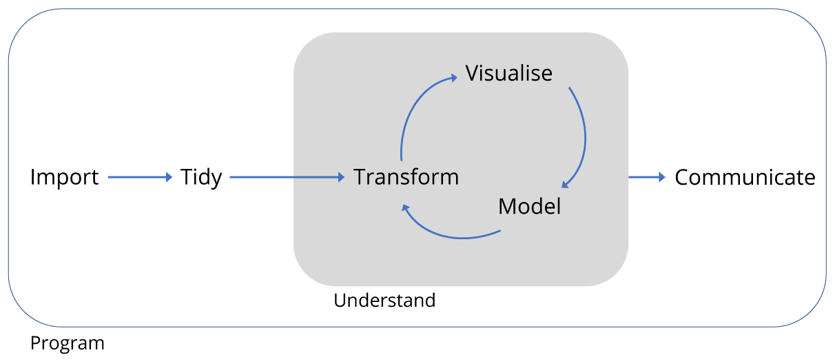
Figure 1.3: Data project workflow.

As shown in Figure 1.3 of typical data analysis workflow, to achieve this aim we need to learn tools that enable us to perform the fundamental tasks of tasks of importing, tidying and often transforming the data. Transformation means for example, selecting a subset of the data to work with, or calculating the mean of a set of observations.

1.2.3 A little goes a long way

Returning to our cat friend in Figure 1.2, one doesn’t need to be an expert programmer to find coding useful. As illustrated in Figure 1.4 there is a whole spectrum of code users from practitioners who are focused on applying some R to their specific problems, to those programmers who develop the R language itself. In reality one may move around on that spectrum as ones interests change over time.

Figure 1.4: The Practitioner-Programmer spectrum

1.3 RStudio

Let’s begin by learning about RStudio, the Integrated Development Environment (IDE).

R is the language and RStudio is software created to facilitate our use of R. They are installed separately. You don’t need RStudio to use R, but you do need R to used RStudio.

We will use R Studio IDE to write code, navigate the files found on our computer, inspect the variables we are going to create, and visualize the plots we will generate. R Studio can also be used for other things (e.g., version control, developing packages, writing Shiny apps) that we don’t have time to cover during this workshop.

R Studio is divided into “Panes”, see Figure 1.5.

When you first open it, there are three panes,the console where you type commands, your environment/history (top-right), and your files/plots/packages/help/viewer (bottom-right).

The environment shows all the R objects you have created or are using, such as data you have imported.

The output pane can be used to view any plots you have created.

Not opened at first start up is the fourth default pane: the script editor pane, but this will open as soon as we create/edit a R script (or many other document types). The script editor is where will be typing much of the time.

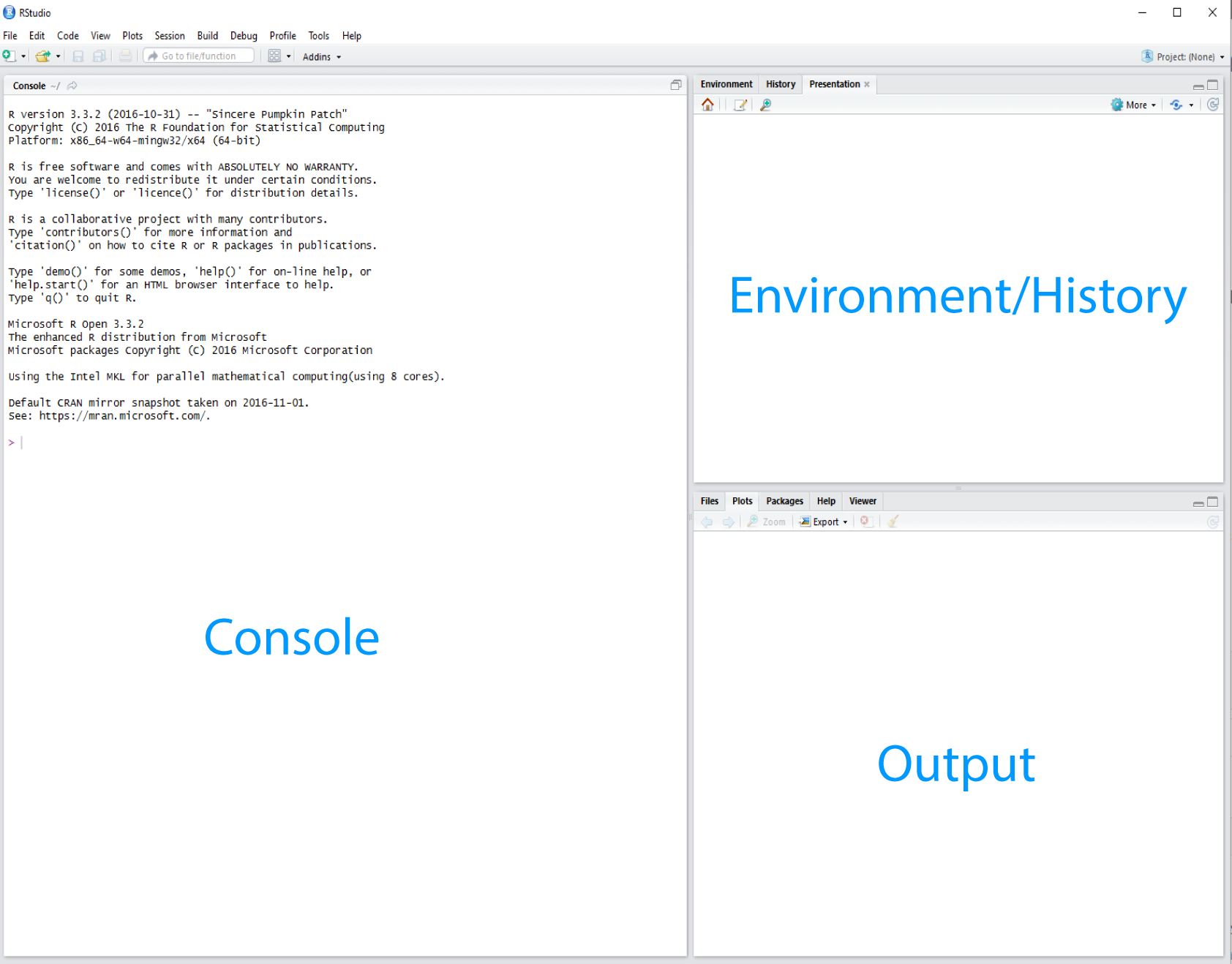
Figure 1.5: The RStudio Integrated Development Environment (IDE).

The placement of these panes and their content can be customized (see menu, R Studio -> Tools -> Global Options -> Pane Layout). One of the advantages of using R Studio is that all the information you need to write code is available in a single window. Additionally, with many short-cuts, auto-completion, and highlighting for the major file types you use while developing in R, R Studio will make typing easier and less error-prone.

RStudio has lots of keyboard short-cuts to make coding quicker and easier. Try to find the menu listing all the keyboard short-cuts, including the short-cut to find the menu!

Time for another philosophical diversion…

1.3.1 What is real?

At the start, we might consider our environment “real” - that is to say the objects we’ve created/loaded and are using are “real”. But it’s much better in the long run to consider our scripts as “real” - our scripts are where we write down the code that creates our objects that we’ll be using in our environment.

As a script is a document, it is reproducible

Or to put it another way: we can easily recreate an environment from our scripts, but not so easily create a script from an environment.

To support this notion of thinking in terms of our scripts as real, we recommend turning off the preservation of workspaces between sessions by setting the Tools > Global Options menu in R studio as shown in Figure 1.6.

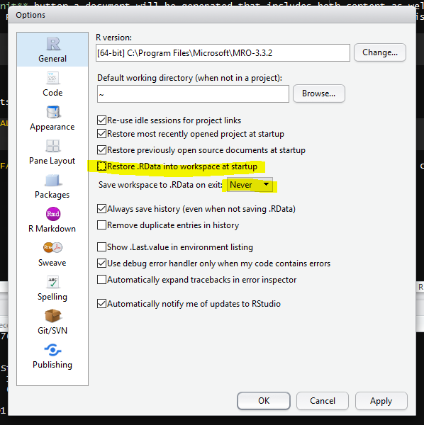
Figure 1.6: Don’t save your workspace, save your script instead.

1.3.2 Where am I?

The part of your computer operating system that manages files and directories (aka folders) is called the file system. This dates back to 1969 and the Unix filesystem.

The idea is that we have a rooted tree, as with phylogenetic rooted trees in biology. From the root all other directories and files exist along paths going back to the root as shown in Figure 1.7.

On Unix based systems such as Apple or Android, the root is denoted with /. On Windows the root is a back slash \. The / or \ is used to to separate directories along the path, denoting a change in the level of the tree

Note: in RStudio the path separator and root is always / regardless of the operating system.

1.3.2.1 Absolute path from the root `/`

In Figure 1.7 the absolute path from the root of surveys.csv is shown. In text this would be /users/alistair/Documents/coding-together-week-02/data/surveys.csv.

This is just a made-up example and the path on your machine will be different.

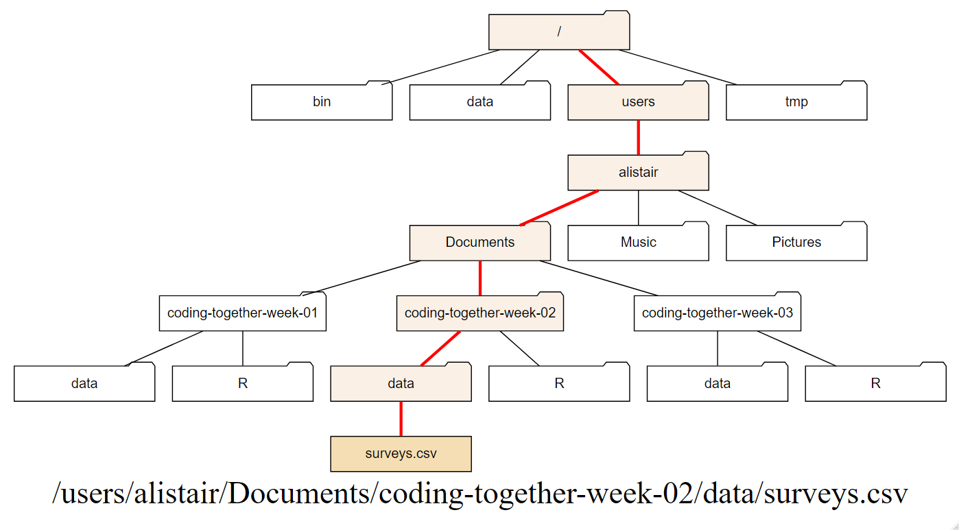
Figure 1.7: The red line shows the absolute path from the root / to surveys.csv.

1.3.2.2 Relative path from where you are `../`

However, we can also consider relative paths, that is relative to where we are working at present.

In Figure 1.8 I imagine that I am working in the R directory in coding-together-week-01 folder. To access the surveys.csv file I have to go up two levels to Documents and then back down three levels. I could use the absolute path, but if I know where surveys.csv is then I can use the short-hand of ../ to go up one level, and then again to go up another, and then back down.

In text from the R directory this is: ../../coding-together-week-02/data/surveys.csv

I don’t reccomend this, it was just to illustrate what a relative path looks like.

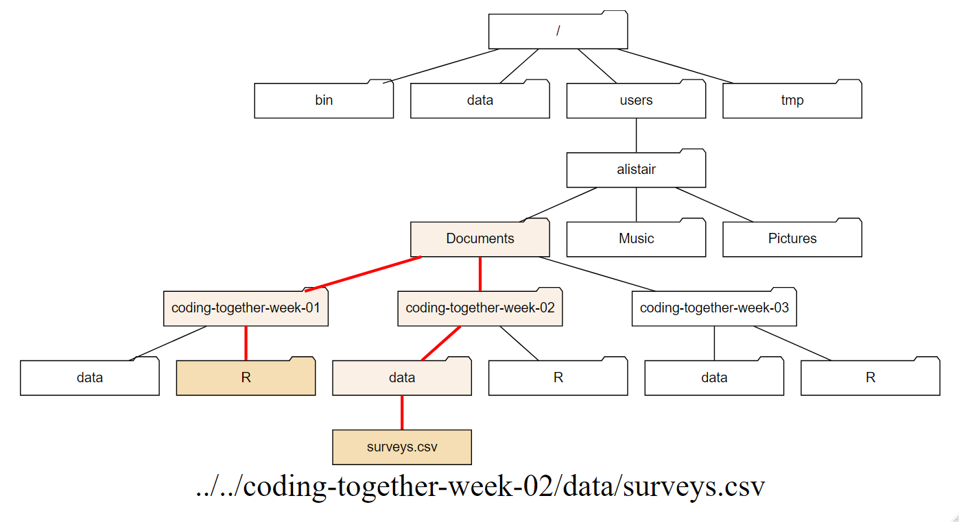
Figure 1.8: The red line represents the relative path from R to surveys.csv

1.3.2.3 Home directory path `~`

The home directory is the part of the file system dedicated to the user - that’s us! - and our data. Usually when we get a new computer we’ll have a home directory with our user name. On Windows machines this will contain My Documents etc. and on an Apple machine it will be Documents etc. On a shared machine each user will get a home directory associated with their user name.

Because we are usually working in our home directory and it’s tiresome to keep typing out paths from the root and it takes up room on the screen, the tilde ~ denotes the path from the root to our home directory.

We can use the ~ to precede the rest of the path to shortcut an absolute path to the root.

Figure 1.9 indicates a home directory path to the surveys.csv with the ~ part in blue and the remaining path in red.

In text this would be: ~/Documents/coding-together-week-02/data/surveys.csv

(ref:home-path) The home directory path to the surveys.csv with the ~ part in blue and the remaining path in red.

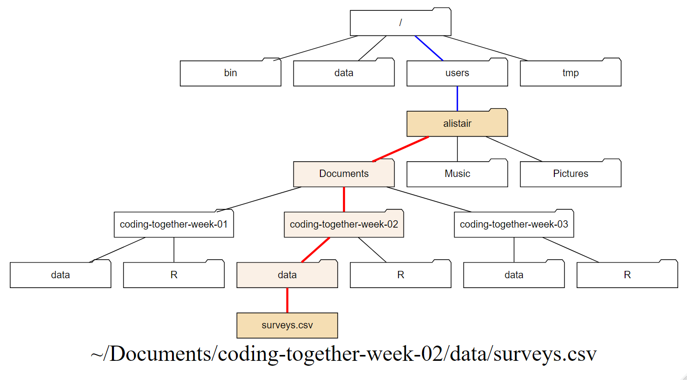
Figure 1.9: (ref:home-path)

1.3.2.4 Working directory

R studio tells you where you are in terms of directory address as shown in Figure 1.10. Here this is a home directory path.

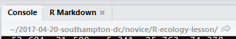
Figure 1.10: Your working directory

It is good practice to keep a set of related data, analyses, and text self-contained in a single folder, called your working directory. All of the scripts within this folder can then use relative paths to files that indicate where inside the project a file is located (as opposed to absolute paths, which point to where a file is on a specific computer). An example directory structure is illustrated in Figure 1.11. Working this way makes it a lot easier to move your project around on your computer. Section 1.7 builds upon this to create a robust workflow for data analysis.

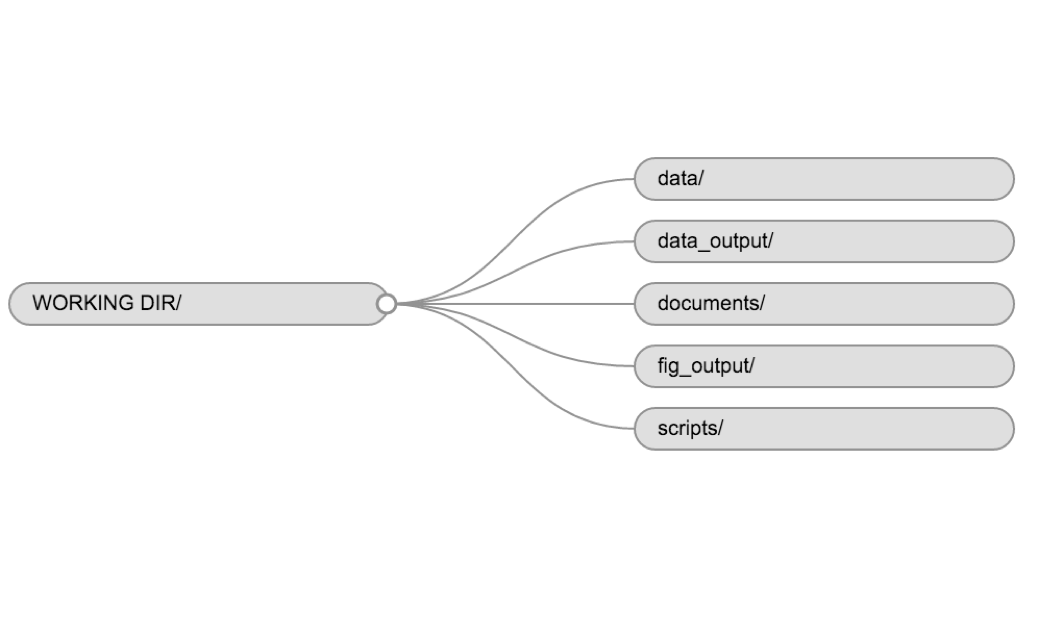
Figure 1.11: A typical directory structure

1.4 Installing and loading packages

Packages are collections of functions, and a function is a piece of code written to perform a specific task, such as installing a package.

Therefore, the function install.packages() is a piece of code written to perform the task of installing packages. We use it by typing install.packages("tidyverse") with the name of the package in quotes inside the round brackets. Here the package is tidyverse. Using the console panel to type this and pressing Enter will run the function.

We of course need to know the name of the packages we are interested in.

Once a package is installed we need to load it into our environment to use it. Loading packages is performed using the library() function. As with installation, we put the name of the package we want to load in between the round brackets like so library(tidyverse). As before this can be done on the console, but we will usually load packages as part of script. Note that we don’t need the quotes for the library function.

Try installing the cowsay package and loading it. It has one function called say() that you can use to create messages with animals.

1.5 Using functions

As stated in 1.4 a function is a piece of code written to perform a specific task. Functions in R have the syntax of the name of the function followed by round brackets. The round brackets are where we type the arguments that the function requires to carry out its task. For example, in 1.4 the function install.packages() requires the name of the package we want to install as arguments.

Many, if not most, functions can take more than one argument. The creators of the function should have given these defaults for the situation where the user provides only one or some arguments. RStudio should prompt you for the arguments as you type, but if you need to see what they are, use the help function ? with the function name in the Console and it will open the help panel or type the function name into the help panel search box.

For example, to find out all the arguments for install.packages() we’d type ?install.packages and press Enter.

Try using say() to say “I are programmer” in the cowsay package and then find out what the arguments you can provide to make it produce different types of message.

1.6 Getting help

1.6.1 Using `?` to access R function help pages

If you need help with a specific R function, let’s say barplot(), you can type the function name without round brackets, with a question mark at the start:

?barplot

1.6.2 Using Google to find R answers

A Google or internet search “R <task>” will often either send you to the appropriate package documentation or a helpful forum question that someone else already asked, such as the RStudio Community or Stack Overflow.

1.6.3 Asking questions

As well as knowing where to ask, the key to get help from someone is for them to grasp your problem rapidly. You should make it as easy as possible to pinpoint where the issue might be.

Try to use the correct words to describe your problem. For instance, a package is not the same thing as a library. Most people will understand what you meant, but others have really strong feelings about the difference in meaning. The key point is that it can make things confusing for people trying to help you. Be as precise as possible when describing your problem.

If possible, try to reduce what doesn’t work to a simple reproducible example otherwise known as a reprex.

For more information on how to write a reproducible example see this article using the reprex package.

1.7 A project orientated workflow

This section is all about how to use R and RStudio to “maximize effectiveness and reduce frustration.”

The above quote is from Jenny Bryan’s article about a project orientated workflow.

The main point here is that how you do things, the workflow, should not be mixed up with the product of the workflow itself.

The product being:

the raw data.
the code needed to produce the results from the raw data.

Ways in which you can mix workflow and product include having lines in your script that set your working directory, or using RStudio to save your environment when you are working.

But why is this a problem?

It’s because your computer isn’t my computer or my laptop isn’t my desktop or I’m now using a Windows machine and I wrote the code two years ago on a Mac.

By hard coding the directory into a script I have ensured my code will only run on the machine in which it was written. Chances are you will want to share your code with someone, either for publication or for them to check your work, or because you are working collaboratively and therefore we need to avoid mixing workflow with product.

Likewise we can’t share environments directly, but we can share the code that creates the environment.

If we organise our analysis into self-contained projects that hold everything needed to perform the analysis. These projects can be shared across machines and the analysis recreated, and thus the workflow is kept separate from the product.

What does this look like in practice?

1.7.1 RStudio Projects

Step one is to use an interactive development environment such as RStudio rather than using R on its own for your analysis.

RStudio contains a facility to keep all files associated with a particular analysis together called, as you might expect from 1.7, a Project.

Creating a Project creates a file .Rproj containing all the information associated with your analysis including the Project location (allowing you to quickly navigate to it), and optionally preserves custom settings and open files to make it easier to resume work after a break. This is also super helpful if you are working on multiple projects as you can switch between them at a click.

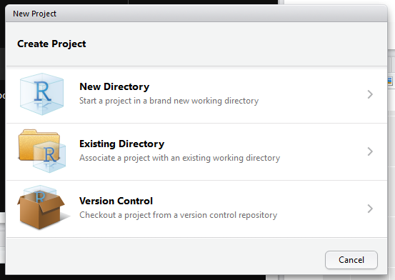
Figure 1.12: Creating a R project

Below, we will go through the steps for creating an Project:

Start R Studio (presentation of R Studio -below- should happen here)
Under the File menu, click on New project, choose New directory, then Empty project
Enter a name for this new folder (or “directory”, in computer science), and choose a convenient location for it. This will be your working directory for the rest of the day (e.g., ~/coding-together)
Click on “Create project”
Under the Files tab on the right of the screen, click on New Folder and create a folder named data within your newly created working directory. (e.g., ~/data)
Create a R notebook (File > New File > R notebook) and save it in your working directory (e.g. 01-coding-together-workshop-02-05-2019.Rmd)
Or create a new R script (File > New File > R script) and save it in your working directory (e.g. 01-coding-together-workshop-02-05-2019.R)

1.7.2 R notebooks and R scripts

R notebooks combine writing text with R code in chunks. The R code chunks are indicated by three backticks and a lowercase r in brackets: ```{r} ```. Text can be formatted using markdown syntax. These are great for doing analysis and report wrting at the same time.

R scripts are text files containing the commands that you would enter into the R console. They are great for containing code you wish to call into another script such as code for a function, or if you are submitting a script as job to run on another computer without the need for RStudio.

1.7.3 Level up with the `here` package

This is a bit more tricky, so you might like to come back to here later, but Jenny Bryan loves the here package by Kirill Müller so much she wrote an ode to it.

In a nutshell, the here() function sets the path implicitly to the top level of the R project you are working in. But what does that mean, and why should I care?

Using the here() function like this:

library(here)

here("data", "file_i_want.csv")

where "data" is the folder containing "file_i_want.csv", the function works out the rest of the path to the folder and file. This is useful if you open the project on different machines where the path is different. here() takes care of things, thus saving you some pain.

1.7.4 Naming things

Jenny Bryan also has three principles for naming things that are well worth remembering.

When you names something, a file or an object, ideally it should be:

Machine readable (no white space, punctuation, upper AND lower-case…)
Human readable (makes sense in 6 months or 2 years time)
Plays well with default ordering (numerical or date order)

We’ll see examples of this as we go along.

1.8 The tidyverse and tidy data

The tidyverse (Wickham 2019) is “an opinionated collection of R packages designed for data science” .

Tidyverse packages contain functions that “share an underlying design philosophy, grammar, and data structures.” It’s this philosophy that makes tidyverse functions and packages relatively easy to learn and use.

Tidy data follows three principals for tabular data as proposed in the Tidy Data paper http://www.jstatsoft.org/v59/i10/paper :

Every variable has its own column.
Every observation has its own row.
Each value has its own cell.

We’ll be using the tidyverse and learning more about tidy data as we go along.

1.9 Atoms of R

Having set ourselves up in RStudio, let’s turn our attention to the language of R itself.

The basic building blocks of how R stores data are called atomic vector types. It’s from these atoms that more complex structures are built. Atomic vectors have one dimension, just like a single row or a single column in a spreadsheet.

The four main atoms of R are:

Doubles: regular numbers, +ve or -ve and with or without decimal places. AKA numerics.
Integers: whole numbers, specified with an upper-case L, e.g. int <- 2L
Characters: Strings of text
Logicals: these store TRUE‘s and FALSE’s’ which are useful for comparisons.

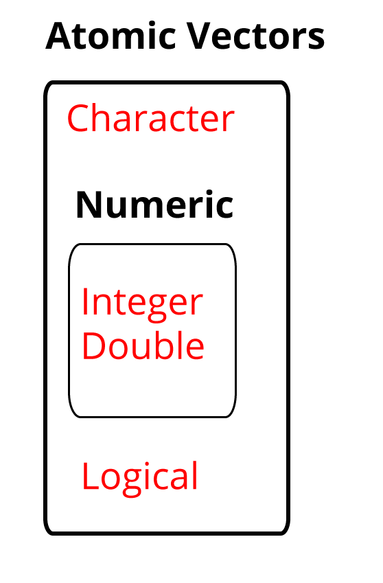
Figure 1.13: The four most used atomic vectors, the building blocks of R

Let’s make a character vector and check the atomic vector type, using the typeof(). This also introduces a very important R function c(). This lower case c stands for combine. So when we have several objects e.g. words or numbers, we can combine them into a vector the length of the number of objects, as illustrated here for a pack of cards:

cards <- c("ace", "king", "queen", "jack", "ten")

cards

## [1] "ace"   "king"  "queen" "jack"  "ten"

typeof(cards)

## [1] "character"

Note here that we see the use of the assignment operator <- to assign our vector on the right as the object cards. We talk more about that in 1.10.

Try creating a vector of numbers from 1 to 10 using the seq() function. Remember to use ?seq if you want to learn more about the function.

1.10 Assigning objects

Objects are just a way to store data inside the R environment. We assign labels to objects using the assignment operator <-

mass_kg <- 55

Read this as “mass_kg is assigned to value 55” in your head. A subtle but important point here is that the object is 55 and the value remains 55 regardless of the label we assign to it. In fact we could assign more than one label to the same object. Another way to think about this is that Bibi is a cat, and remains a cat even if I call her Princess when she refuses to go out in the rain.

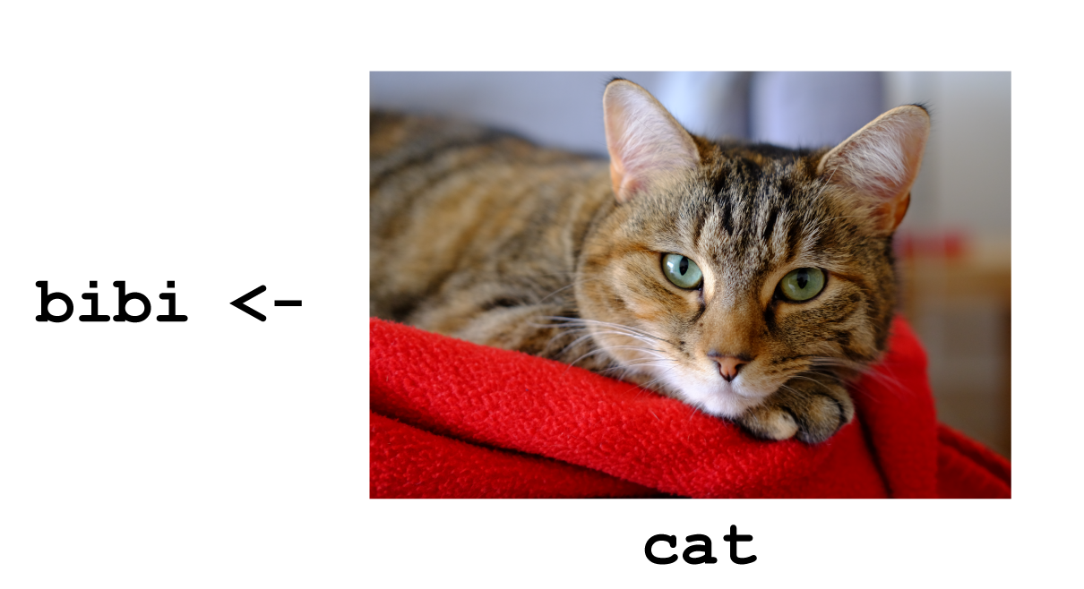
Figure 1.14: Bibi remains a cat even if I call her Princess when she refuses to go out in the rain.

Using <- can be annoying to type, so use RStudio’s keyboard short cut: Alt + - (the minus sign) to make life easier.

Many people ask why we use this assignment operator when we can use = instead?

Colin Fay had a Twitter thread on this subject, but the reason I favour most is that it provides clarity. The arrow points in the direction of the assignment (it is actually possible to assign in the other direction too) and it distinguishes between creating an object in the workspace and assigning a value inside a function.

Object name style is a matter of choice, but must start with a letter and can only contain letters, numbers, _ and .. We recommend using descriptive names and using _ between words. Some special symbols cannot be used in variable names, so watch out for those.

So here we’ve used the name to indicate its value represents a mass in kilograms. Look in your environment pane and you’ll see the mass_kg object containing the (data) value 55.

We can inspect an object by typing it’s name:

mass_kg

## [1] 55

What’s wrong here?

mass_KG

Error: object 'mass_KG' not found

This error illustrates that typos matter, everything must be precise and mass_KG is not the same as mass_kg. mass_KG doesn’t exist, hence the error.

Let’s use seq() to create a sequence of numbers, and at the same time practice tab completion.

Start typing se in the console and you should see a list of functions appear, add q to shorten the list, then use the up and down arrow to highlight the function of interest seq() and hit Tab to select. This is tab completion.

RStudio puts the cursor between the parentheses to prompt us to enter some arguments. Here we’ll use 1 as the start and 10 as the end:

seq(1,10)

##  [1]  1  2  3  4  5  6  7  8  9 10

If we left off a parentheses to close the function, then when we hit enter we’ll see a + indicating RStudio is expecting further code. We either add the missing part or press Escape to cancel the code.

Let’s call a function and make an assignment at the same time. Here we’ll use the base R function seq() which takes three arguments: from, to and by.

Read the following code as "assign my_sequence to an object that stores a sequence of numbers from 2 to 20 by intervals of 2.

my_sequence <- seq(2,20,2)

This time nothing was returned to the console, but we now have an object called my_sequence in our environment.

1.10.1 Indexing and subsetting

If we want to access and subset elements of my_sequence we use square brackets [] and the index number. Indexing in R starts at 1 such that 1 is the index of the first element in the sequence, element 1 having the the value of 2.

For example element five would be subset by:

my_sequence[5]

## [1] 10

Here the number five is the index of the vector, not the value of the fifth element. The value of the fifth element is 10.

And returning multiple elements uses a colon :, like so

my_sequence[5:8]

## [1] 10 12 14 16

1.11 Lists, matrices and arrays

Lists also group data into one dimensional sets of data. The difference being that list group objects instead of individual values, such as several atomic vectors.

For example, let’s make a list containing a vector of numbers and a character vector

list_1 <- list(1:110,"R")

list_1

## [[1]]
##   [1]   1   2   3   4   5   6   7   8   9  10  11  12  13  14  15  16  17  18
##  [19]  19  20  21  22  23  24  25  26  27  28  29  30  31  32  33  34  35  36
##  [37]  37  38  39  40  41  42  43  44  45  46  47  48  49  50  51  52  53  54
##  [55]  55  56  57  58  59  60  61  62  63  64  65  66  67  68  69  70  71  72
##  [73]  73  74  75  76  77  78  79  80  81  82  83  84  85  86  87  88  89  90
##  [91]  91  92  93  94  95  96  97  98  99 100 101 102 103 104 105 106 107 108
## [109] 109 110
## 
## [[2]]
## [1] "R"

Note the double brackets to indicate the list elements, i.e. element one is the vector of numbers and element two is a vector of a single character.

We won’t be working with lists a great deal in these workshops, but they are a flexible way to store data of different types in R.

Accessing list elements uses double square brackets syntax, for example list_1[[1]] would return the first vector in our list.

And to access the first element in the first vector would combine double and single square brackets like so: list_1[[1]][1].

Don’t worry if you find this confusing, everyone does when they first start with R. Hadley Wickham tweeted an image to illustrate list indexing shown in 1.15.

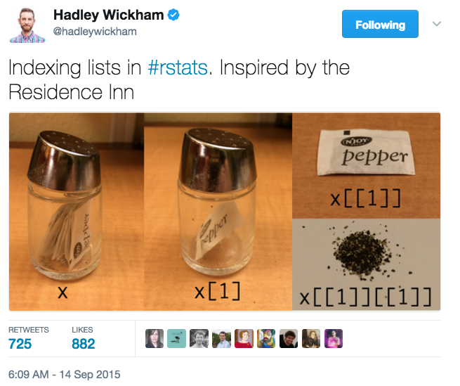
Figure 1.15: List indexing by Hadley Wickham

Lists alongside NULL which indicates the absence of a vector, complete the set of base vectors in R as illustrated in 1.16.

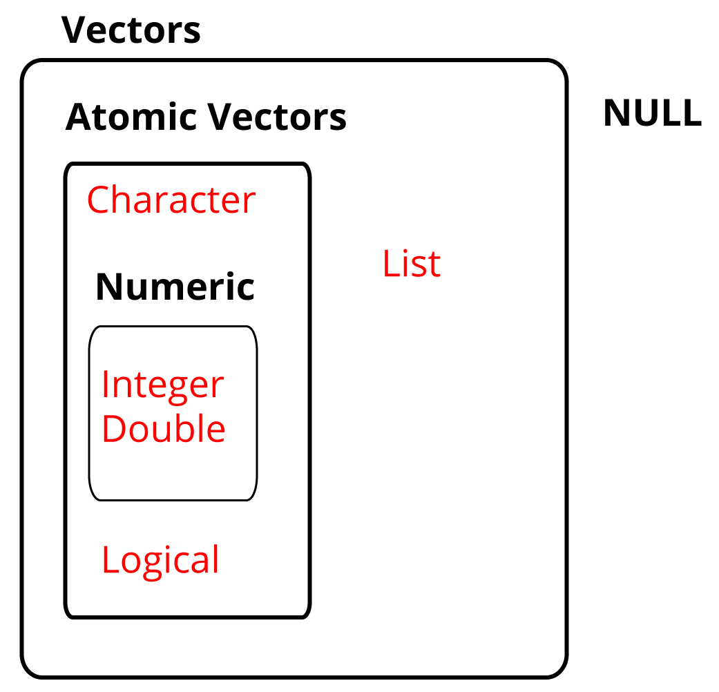
Figure 1.16: The base vectors in R.

1.11.1 Matrices and arrays

Matrices store values in a two dimensional array, whilst arrays can have n dimensions. We won’t be using these either, but they are also valid R objects.

1.12 Factors

Factors are Rs way of storing categorical information such as eye colour or car type. A factor is something that can only have certain values, and can be ordered (such as low,medium,high) or unordered such as types of fruit.

Factors are useful as they code string variables such as “red” or “blue” to integer values e.g. 1 and 2, which can be used in statistical models and when plotting, but they are confusing as they look like strings.

Factors look like strings, but behave like integers.

Historically R converts strings to factors when we load and create data, but it’s often not what we want as a default. Fortunately, in the tidyverse strings are not treated as factors by default.

1.13 Data frames

For data analysis in R, we mostly be using data frames.

Data frames are two dimensional versions of lists, and this is form of storing data we are going to be using. In a data frame each atomic vector type becomes a column, and a data frame is formed by columns of vectors of the same length. Each column element must be of the same type, but the column types can vary.

Figure 1.17 shows an example data frame we’ll refer to as saved as the object df consisting of three rows and three columns. Each column is a different atomic data type of the same length.

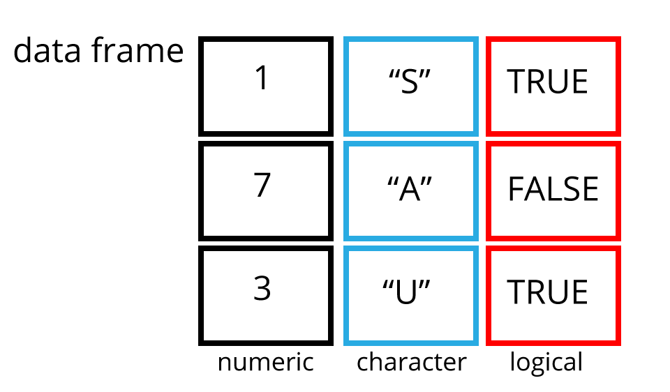
Figure 1.17: An example data frame df.

To create the data frame 1.17 we can use the data.frame() function in conjunction with the c() function to make the individual atomic vectors that comprise the data frame as follows. Note that I am naming the vectors as I make the data frame after the type of vector e.g. numeric_vector = c(1,7,3). Also, as this is a base R function I need to tell the function not to treat the character strings as categorical data using stringsAsFactors = FALSE

df <- data.frame(numeric_vector = c(1,7,3), 
                 character_vector = c("S","A","U"),
                 logical_vector = c(TRUE,FALSE,TRUE), 
                 stringsAsFactors = FALSE)

df

##   numeric_vector character_vector logical_vector
## 1              1                S           TRUE
## 2              7                A          FALSE
## 3              3                U           TRUE

Packages in the tidyverse create a modified form of data frame called a tibble. You can read about tibbles here. One advantage of tibbles is that they don’t default to treating strings as factors. We deal with transforming data frames in chapters 2 and 3.

Here’s what the code to make the same data frame as before as a tibble looks like. Note how we get more information from a tibble when it is returned to the Console, it tells us what the dimensions are, and what type of vectors it contains.

df <- tibble(numeric_vector = c(1,7,3), 
                 character_vector = c("S","A","U"),
                 logical_vector = c(TRUE,FALSE,TRUE))

df

## # A tibble: 3 x 3
##   numeric_vector character_vector logical_vector
##            <dbl> <chr>            <lgl>         
## 1              1 S                TRUE          
## 2              7 A                FALSE         
## 3              3 U                TRUE

Sub-setting data frames can also be done with square bracket syntax, but as we have both rows and columns, we need to provide index values for both row and column.

For example df[1,2] means return the value of df row 1, column 2. This corresponds with the value A.

We can also use the colon operator to choose several rows or columns, and by leaving the row or column blank we return all rows or all columns.

# Subset rows 1 and 2 of column 1
df[1:2,1]

# Subset all rows of column 3
df[,3]

Don’t worry too much about this for now, we won’t be doing to much of this in these lessons, but it’s worth being aware of this syntax.

1.13.1 Attributes

An attribute is a piece of information you can attach to an object, such as names or dimensions. Attributes such as dimensions are added when we create an object, but others such as names can be added.

Let’s look at the mpg data frame dimensions:

# mpg has 234 rows (observations) and 11 columns (variables)
dim(mpg)

## [1] 234  11

1.14 Plotting data

One of the most useful and important parts of any data analysis is plotting data. We’ll be spending a whole lesson on it in chapter 4, but to give you an example, we’ll use the ggplot2 package as an introduction to automating a task in code, and as a tool for understanding data.

ggplot2 implements the grammar of graphics, for describing and building graphs. The idea being that we construct a plot in the following way:

Call the ggplot() function to create a graph.
Pass our data as the first argue to the ggplot() function.
Then pass some arguments to the aesthetics function aes() inside the gpplot() which tell ggplot how to plot the data e.g. which data goes on the x and y axis.
Then we follow the ggplot function with a + sign to indicate we are going to add more code, followed by a geometric object function, a geom which maps the data to type of plot we want to make e.g. a histogram or scatter plot.

Don’t worry if this sounds confusing, it becomes clear with practice and all plots follow this grammar.

We’ll use the mpg dataset that comes with the tidyverse to examine the question do cars with big engines use more fuel than cars with small engines?

Try ?mpg to learn more about the data.

Engine size in litres is in the displ column.
Fuel efficiency on the highway in miles per gallon is given in the hwy column.

To create a plot of engine size displ (x-axis) against fuel efficiency hwy (y-axis) we do the following:

Now try extending this code to include to add a colour aesthetic to the the aes() function, let colour = class, class being the vehicle type. This should create a plot with as before but with the points coloured according to the vehicle type to expand our understanding.

ggplot(data = mpg) + 
  geom_point(mapping = aes(x = displ, y = hwy, colour = class))

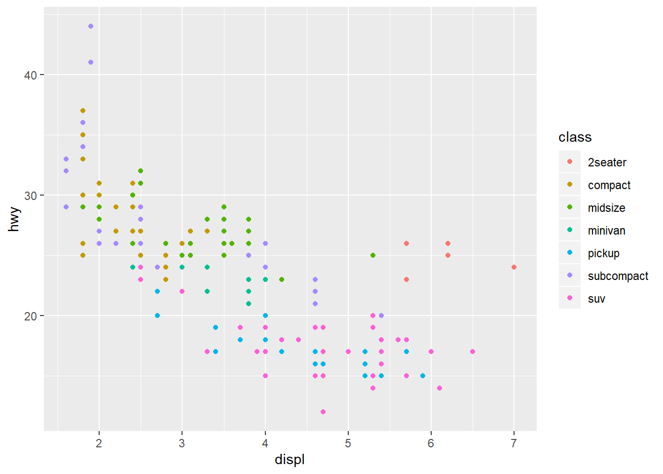
Now we can see that as we might expect, bigger cars such as SUVs tend to have bigger engines and are also less fuel efficient, but some smaller cars such as 2-seaters also have big engines and greater fuel efficiency. Hence we have a more nuanced view with this additional aesthetic.

Check out the ggplot2 documentation for all the aesthetic possibilities (and Google for examples): http://ggplot2.tidyverse.org/reference/

So now we have re-usable code snippet for generating plots in R:

ggplot(data = <DATA>) + 
  <GEOM_FUNCTION>(mapping = aes(<MAPPINGS>))

Concretely, in our first example <DATA> was mpg, the <GEOM_FUNCTION> was geom_point() and the arguments we supplies to map our aesthetics <MAPPINGS> were x = displ, y = hwy.

As we can use this code for any tidy data set, hopefully you are beginning to see how a small amount of code can do a lot.

1.15 Exporting data

We’ll spend more time on getting data in and out of our R environment in the next chapter 3, but just to wrap this lesson up let’s imagine we wanted to export our plot and data for a colleague or presentation.

1.15.1 readr

To export tibbles and data frames, we’ll use the readr package, and the write_excel_csv() function. This creates a table in comma separated variable format that can opened by spreadsheet software such as excel.

As it is a function is has round brackets and the main arguments we pass are the object containing the data we want to output and the name of the file and the location we want to write the file to.

write_excel_csv(df, "outputs/example-data-02-05-2019.csv")

Here we are writing the df data frame as a csv file to the outputs folder and a file called example-data-02-05-2019.csv.

1.15.2 ggsave

If we want to save the last plot we made in ggplot2 we can use the ggsave() function

We tell ggsave() the filename, and it will save it as that type depending on how we name the file. For example if we use file.pdf it will save a PDF and if we use file.jpeg it will save a jpeg.

Check out ?ggsave or the line above for more options.

To save our last plot for example:

ggsave("outputs/example-plot-02-05-2019.pdf")

1.15.3 Exercise

Create a new project called ‘coding-assessment-01’

Create two folders in this project: R and outputs

Create a R script using best naming practices i.e. name-date.R

In the script, write some comments at the top e.g. name, date, description

Create a tibble comprising of a character vector, a numeric vector

Install and load the dslabs package and create a density plot with ggplot2 using the heights dataset, using the x = height variable and fill = sex to create a density plot ggplot(data = heights, aes(x =height, fill = sex)) + geom_density()

Save the plot as pdf and the tibble as csv file to the output folder.

References

Ihaka, Ross, and Robert Gentleman. 1996. “R: A Language for Data Analysis and Graphics.” Journal of Computational and Graphical Statistics 5 (3): 299–314.

Wickham, Hadley. 2019. Tidyverse: Easily Install and Load the ’Tidyverse’. https://CRAN.R-project.org/package=tidyverse.