3 Data wrangling II
Following on from chapter 2 this lesson deals with some
common tidying problems with data using the tidyr package . By the end of this chapter the learner
will:
- have learnt how to transform rows and columns to reorganise data
- have learnt some ways to deal with missing values
- have learnt how to join data contained in separate tables into a single table
3.1 Reshaping data with pivots
As you will recall tidy data means that in a table:
- Every variable has its own column.
- Every observation has its own row.
- Each value has its own cell.
Two common problems making your data untidy are that:
- A single variable is spread across multiple colummns.
- A single observation is distributed across multiple rows.
In the first case the column names are actually the variable we are interested in, making our table wide.
In the second case, the observation is contained in several rows instead of a single row, making our table long.
Hence tidyr has functions that pivot (as in turning) a table from wide-to-long by reducing the number of columns and increasing the number of rows. Or from long-to-wide by reducing the number of rows and increasing the number of columns.
Usually, the hard part is identifying in a dataset our variables and our observations, as it is not always obvious which is which.
3.1.1 tidyr::pivot_longer
First we’ll consider the case when our variable has been recorded as column names by returning to a version of the Portal surveys data.
A table containing the mean weight of 10 rodent species on each plot from the rodent survey data
can be read directly into a surveys_spread object using the code below.
Feel free to explore the data, and snapshot is shown in Figure 3.1.
Imagine that we recorded the mean weight of each rodent species on a plot in the field. It makes sense to put the species as column headings, along with the plot id and then record the values in each cell.
However, really our variables of interest are the rodent species and our observational units, the rows, should contain the mean weight for a rodent species in a plot. Hence we need to reduce the number of columns and create a longer table.
To do this we pivot_longer() by using names_to = "genus" to create a new genus
variable for the exisiting column heading, and values_to = "mean_weight" to create
a variable mean_weight for the values. We put a minus sign before the
variable -plot_id to tell the function not to use these values in the new variable column.
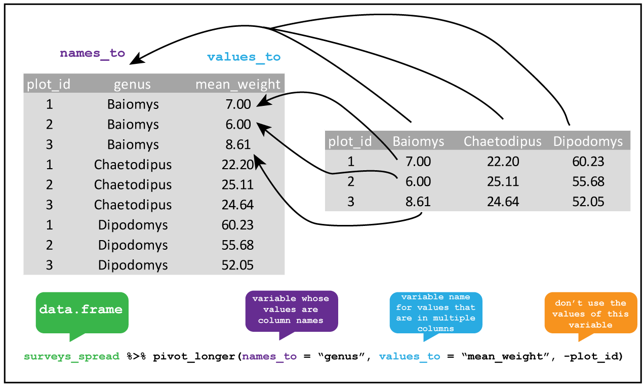
Figure 3.1: tidyr::pivot_longer The genus of the rodents have been used as column headings for the weights of each animal. By creating new variables genus which takes the column names, and another variable mean_weight which takes the cell values, and but not the plot_id column we pivot from a wide table to a long table.
## # A tibble: 240 x 3
##    plot_id genus           mean_weight
##      <dbl> <chr>                 <dbl>
##  1       1 Baiomys                7
##  2       1 Chaetodipus           22.2
##  3       1 Dipodomys             60.2
##  4       1 Neotoma              156.
##  5       1 Onychomys             27.7
##  6       1 Perognathus            9.62
##  7       1 Peromyscus            22.2
##  8       1 Reithrodontomys       11.4
##  9       1 Sigmodon              NA
## 10       1 Spermophilus          NA
## # … with 230 more rows
3.1.2 tidyr::pivot_wider
If we wanted to go the other way, from wide to long, then we need to take values from a single column to become variables names of multiple columns, populated with values from an existing variable.
A version of the wide table in Figure 3.2 can be downloaded
into our environment and assigned as surveys_gw as before.
This time we use pivot_wider() with the arguments names_from for the column
we want to use to create variables, and values_from for the column
whose values we want populate our new variable columns with.
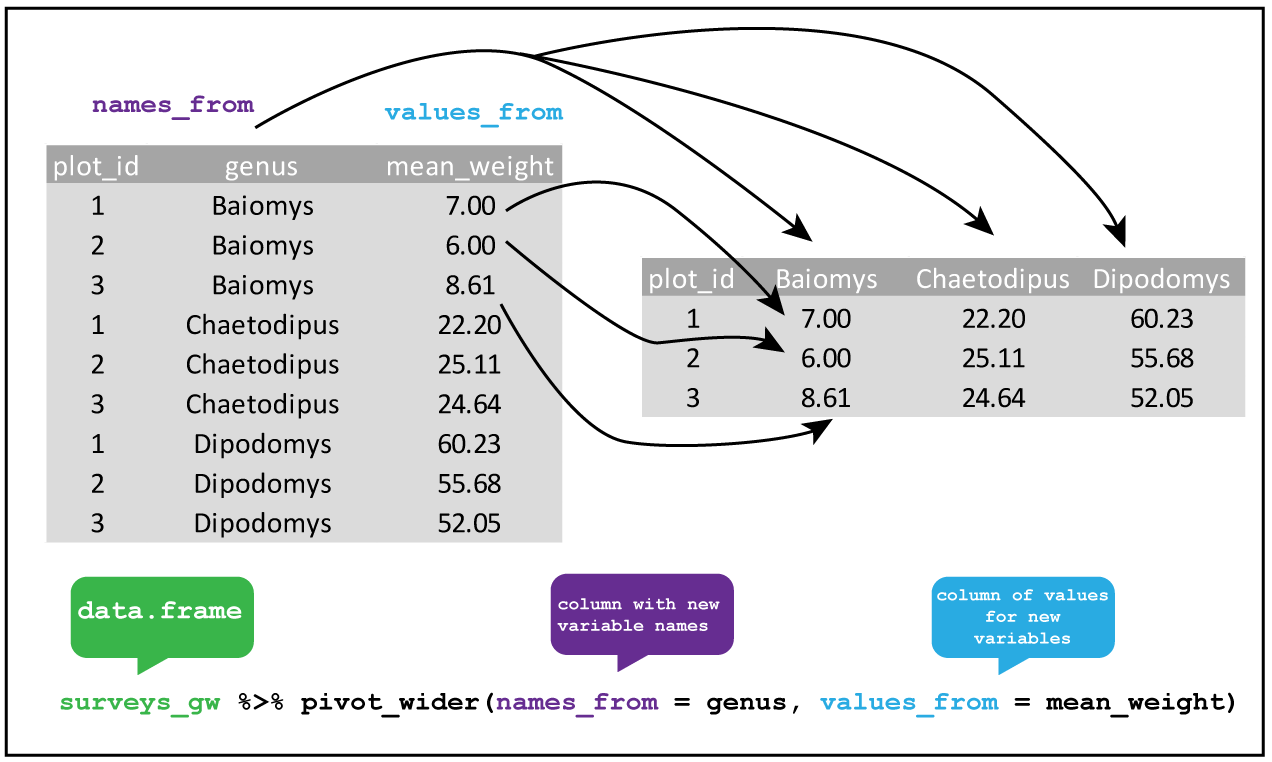
Figure 3.2: tidyr::pivot_wider From long table surveys_gw the genus column contains the values that become variables using names_from and the mean_weight column contains the values that fill the new columns using values_from in the pivot from long to wide.
## # A tibble: 24 x 11
##    plot_id Baiomys Chaetodipus Dipodomys Neotoma Onychomys Perognathus
##      <dbl>   <dbl>       <dbl>     <dbl>   <dbl>     <dbl>       <dbl>
##  1       1    7           22.2      60.2    156.      27.7        9.62
##  2       2    6           25.1      55.7    169.      26.9        6.95
##  3       3    8.61        24.6      52.0    158.      26.0        7.51
##  4       5    7.75        18.0      51.1    190.      27.0        8.66
##  5      18    9.5         26.8      61.4    149.      26.6        8.62
##  6      19    9.53        26.4      43.3    120       23.8        8.09
##  7      20    6           25.1      65.9    155.      25.2        8.14
##  8      21    6.67        28.2      42.7    138.      24.6        9.19
##  9       4   NA           23.0      57.5    164.      28.1        7.82
## 10       6   NA           24.9      58.6    180.      25.9        7.81
## # … with 14 more rows, and 4 more variables: Peromyscus <dbl>,
## #   Reithrodontomys <dbl>, Sigmodon <dbl>, Spermophilus <dbl>
3.2 Missing values
In R missing values are represented as NA (or NaN for an undefined mathematical
operation such as dividing by zero).
As discussed in R4DS values can be missing in two ways:
- Explicitly, i.e. flagged with NA.
- Implicitly, i.e. simply not present in the data.
If we had a subset of the surveys data that looked like this table:
# Create a table with missing values
surveys_ms <- tibble(year = c(1991,1991,1991,1991,1992,1992,1992),
                     qtr = c(1,2,3,4,1,2,4),
                     mean_weight = c(3.75,2.50,NA,8.50,7.50,2.25,2.50))

surveys_ms
## # A tibble: 7 x 3
## year qtr mean_weight
## <dbl> <dbl> <dbl>
## 1 1991 1 3.75
## 2 1991 2 2.5
## 3 1991 3 NA
## 4 1991 4 8.5
## 5 1992 1 7.5
## 6 1992 2 2.25
## 7 1992 4 2.5Then we can see that in the third quarter of 1991, no data was recorded by the
explicit NA value. However the third quarter of 1992 is missing altogether,
hence it is implicitly missing.
Another issue is that explicit missing values
are often recorded in real data in various ways e.g. an empty cell or as a dash.
We can’t cover all cases, but the general advice is to do some manual inspection
of your data in addition to using R to understand how missing values have been
recorded if there are any. In an ideal world data comes with a “code book” that
explains the data, but this often doesn’t happen.
Functions such as read_csv() allow you to
supply a vector of values representing NA which will convert these values in
your input to NAs.
Once you have identified missing values, in general there two ways to deal with them:
- Drop incomplete observations
- Complete the missing observations: fill or impute values.
See also tidyr functions for missing values.
3.2.1 Checking for explicit missing values using R
In addition to manual inspection, one way to check for explicit missing
values coded as NA in your data frame is to use the is.na() function which
returns a logical TRUE or FALSE vector of values.
Using this to check a single variable could be done by combining it with select()
for example using surveys_ms:
## mean_weight
## [1,] FALSE
## [2,] FALSE
## [3,] TRUE
## [4,] FALSE
## [5,] FALSE
## [6,] FALSE
## [7,] FALSEOr with filter() to return the row where there is a missing value
for mean_weight.
## # A tibble: 1 x 3
## year qtr mean_weight
## <dbl> <dbl> <dbl>
## 1 1991 3 NAA more complicated use would be to combine is.na() with another function such
sum() to provide the total number of missing values for a variable, or to
combine sum() with complete.cases() to check each row for for missing values.
For example, to find the number of observations (rows) in surveys with no missing values:
## [1] 30676And for a single variable, we could extend our use of select:
## [1] 1Extending this find the missing values per variable in a whole data frame
requires introducing more syntax and the use of a map function from the purr
package. (Base R can also do this, but we’re staying in the tidyverse where possible).
The idea here is that we want to do the same calculation mapped across each variable. The calculation here being count the number of missing values in each column.
We pipe surveys to the map_dfr() function where dfr means return a data frame.
The ~ represents formula, meaning “depends upon”, such that sum(is.na(.)) where .
represents the input variable, depends upon the variables in surveys.
The map function then does this for each variable in the surveys dataframe
and returns the output as a data frame. I’ve piped the output to glimpse() for
readability.
In words what this syntax is saying is “take the surveys dataframe and for
each column check if each value is NA, then sum the number of NAs in each
column and return the totals for all the columns as a dataframe.”
This is pretty complicated if you’ve never seen this before, but hopefully you can follow the idea.
This could be combined with filter() or select() prior to the map function
if you wanted to subset the data further for example.
See R4DS map functions for more details.
## Observations: 1
## Variables: 13
## $ record_id <int> 0
## $ month <int> 0
## $ day <int> 0
## $ year <int> 0
## $ plot_id <int> 0
## $ species_id <int> 0
## $ sex <int> 1748
## $ hindfoot_length <int> 3348
## $ weight <int> 2503
## $ genus <int> 0
## $ species <int> 0
## $ taxa <int> 0
## $ plot_type <int> 0As we might expect the missing values are all for variables that record measurements for the rodents.
3.2.2 Dropping missing values
The simplest solution to observations with missing values is to drop those
from the data set. If it makes sense to do this, then tidyr::drop_na() makes
it easy to do this. Note: This will create implicit missing values.
In Section 3.2.1 we found 30,676 rows with no missing values
by using complete.cases() on the surveys data of 34,786 observations.
Therefore we expect passing surveys to drop_na() will return a dataframe
of 30,676 observations:
## Observations: 30,676
## Variables: 13
## $ record_id <dbl> 845, 1164, 1261, 1756, 1818, 1882, 2133, 2184, 2406, …
## $ month <dbl> 5, 8, 9, 4, 5, 7, 10, 11, 1, 5, 5, 7, 10, 11, 1, 2, 3…
## $ day <dbl> 6, 5, 4, 29, 30, 4, 25, 17, 16, 18, 18, 8, 1, 23, 25,…
## $ year <dbl> 1978, 1978, 1978, 1979, 1979, 1979, 1979, 1979, 1980,…
## $ plot_id <dbl> 2, 2, 2, 2, 2, 2, 2, 2, 2, 2, 2, 2, 2, 2, 2, 2, 2, 2,…
## $ species_id <chr> "NL", "NL", "NL", "NL", "NL", "NL", "NL", "NL", "NL",…
## $ sex <chr> "M", "M", "M", "M", "M", "M", "F", "F", "F", "F", "F"…
## $ hindfoot_length <dbl> 32, 34, 32, 33, 32, 32, 33, 30, 33, 31, 33, 30, 34, 3…
## $ weight <dbl> 204, 199, 197, 166, 184, 206, 274, 186, 184, 87, 174,…
## $ genus <chr> "Neotoma", "Neotoma", "Neotoma", "Neotoma", "Neotoma"…
## $ species <chr> "albigula", "albigula", "albigula", "albigula", "albi…
## $ taxa <chr> "Rodent", "Rodent", "Rodent", "Rodent", "Rodent", "Ro…
## $ plot_type <chr> "Control", "Control", "Control", "Control", "Control"…drop_na() can accept variables arguments, meaning only the observations with
missing values in those columns will be dropped.
For example, here we drop only missing weight observations, so the rows which
have missing values for hindfoot_length or sex are kept.
## Observations: 32,283
## Variables: 13
## $ record_id <dbl> 588, 845, 990, 1164, 1261, 1453, 1756, 1818, 1882, 21…
## $ month <dbl> 2, 5, 6, 8, 9, 11, 4, 5, 7, 10, 11, 1, 5, 5, 7, 10, 1…
## $ day <dbl> 18, 6, 9, 5, 4, 5, 29, 30, 4, 25, 17, 16, 18, 18, 8, …
## $ year <dbl> 1978, 1978, 1978, 1978, 1978, 1978, 1979, 1979, 1979,…
## $ plot_id <dbl> 2, 2, 2, 2, 2, 2, 2, 2, 2, 2, 2, 2, 2, 2, 2, 2, 2, 2,…
## $ species_id <chr> "NL", "NL", "NL", "NL", "NL", "NL", "NL", "NL", "NL",…
## $ sex <chr> "M", "M", "M", "M", "M", "M", "M", "M", "M", "F", "F"…
## $ hindfoot_length <dbl> NA, 32, NA, 34, 32, NA, 33, 32, 32, 33, 30, 33, 31, 3…
## $ weight <dbl> 218, 204, 200, 199, 197, 218, 166, 184, 206, 274, 186…
## $ genus <chr> "Neotoma", "Neotoma", "Neotoma", "Neotoma", "Neotoma"…
## $ species <chr> "albigula", "albigula", "albigula", "albigula", "albi…
## $ taxa <chr> "Rodent", "Rodent", "Rodent", "Rodent", "Rodent", "Ro…
## $ plot_type <chr> "Control", "Control", "Control", "Control", "Control"…3.2.3 Completing missing values
There are numerous ways to complete missing values, but what they generally
have in common is the approach of guessing the missing value based on existing information, otherwise known as imputation.
Here we’ll cover a couple of ways to do it with dplyr and tidyr functions.
First, let’s deal with implicit missing values using tidyr::complete().
Imagine we have the table surveys_ms which is missing the value
for the mean_weight for the third quarter of 1991 and all observations
for the third quarter of 1992:
## # A tibble: 7 x 3
##    year   qtr mean_weight
##   <dbl> <dbl>       <dbl>
## 1  1991     1        3.75
## 2  1991     2        2.5
## 3  1991     3       NA
## 4  1991     4        8.5
## 5  1992     1        7.5
## 6  1992     2        2.25
## 7 1992 4 2.5To add the row for the third quarter of 1992 we use complete() with the
year and qtr variables as arguments. The function finds all the unique
combinations of year and qtr and then adds any that are missing to create
a complete set of observations for 1991 and 1992 with explicit missing values.
## # A tibble: 8 x 3
## year qtr mean_weight
## <dbl> <dbl> <dbl>
## 1 1991 1 3.75
## 2 1991 2 2.5
## 3 1991 3 NA
## 4 1991 4 8.5
## 5 1992 1 7.5
## 6 1992 2 2.25
## 7 1992 3 NA
## 8 1992 4 2.5Next let’s consider a complete table surveys_ic with an explicit missing value for
the species_id.
surveys_ic <- tibble(species_id = c("DM","DM",NA,"DS","DS","DS"),
mean_weight = c(3.75,2.50,8.50,7.50,5.50,2.50))
surveys_ic## # A tibble: 6 x 2
## species_id mean_weight
## <chr> <dbl>
## 1 DM 3.75
## 2 DM 2.5
## 3 <NA> 8.5
## 4 DS 7.5
## 5 DS 5.5
## 6 DS 2.5In this case we might reasonably assume that the missing value is DM as we
have six observations on two species.
We can use tidyr::fill() to replace NA with the last non-missing value for
species_id. This is also known as last observation carried forward.
Passing species_id to fill() completes the table:
## # A tibble: 6 x 2
## species_id mean_weight
## <chr> <dbl>
## 1 DM 3.75
## 2 DM 2.5
## 3 DM 8.5
## 4 DS 7.5
## 5 DS 5.5
## 6 DS 2.5Another common strategy is to impute missing values by using the mean or the median of exisiting values for the same variable.
We can do that using dplyr::coalesce() which is a function that finds the
first non-missing value in a variable and then replaces it using the second
argument.
For example, if we return to surveys_ms we used complete() to complete
the observations, but we have two NAs in the mean_weight column.
Let’s impute the missing values bt using the median value for mean_weight to
replace the NA values.
We can mutate() to overwrite the mean_weight variable (be careful when
you do this!) using coalesce() with mean_weight as the first argument to look
for missing values, and then the median() function is used to replace the missing
values with the median mean_weight, remembering to remove NA.
surveys_ms %>%
complete(year,qtr) %>%
mutate(mean_weight = coalesce(mean_weight,
median(mean_weight, na.rm = TRUE)))## # A tibble: 8 x 3
## year qtr mean_weight
## <dbl> <dbl> <dbl>
## 1 1991 1 3.75
## 2 1991 2 2.5
## 3 1991 3 3.12
## 4 1991 4 8.5
## 5 1992 1 7.5
## 6 1992 2 2.25
## 7 1992 3 3.12
## 8 1992 4 2.5This gives us a complete table with . Whether it makes sense to do this is another question, and you should think carefully about your missing value strategy as it will influence your final output and conclusions.
Let’s repeat part of the analysis we did to find the mean_weight, and now
mean_hindfoot, for the full surveys dataset, but this time we’ll
complete the table by imputing values and compare the result to the result when
we drop the observations with missing values.
For simplicity, let’s just look at kangaroo rats. Here I introduce the %in%
operator with filter and vector containing the species_id for the kangaroo
rats.
This leaves 16,127 observations.
## Observations: 16,127
## Variables: 13
## $ record_id       <dbl> 3, 226, 233, 245, 251, 257, 259, 268, 346, 350, 354, …
## $ month           <dbl> 7, 9, 9, 10, 10, 10, 10, 10, 11, 11, 11, 11, 12, 12, …
## $ day             <dbl> 16, 13, 13, 16, 16, 16, 16, 16, 12, 12, 12, 12, 10, 1…
## $ year            <dbl> 1977, 1977, 1977, 1977, 1977, 1977, 1977, 1977, 1977,…
## $ plot_id         <dbl> 2, 2, 2, 2, 2, 2, 2, 2, 2, 2, 2, 2, 2, 2, 2, 2, 2, 2,…
## $ species_id      <chr> "DM", "DM", "DM", "DM", "DM", "DM", "DM", "DM", "DM",…
## $ sex             <chr> "F", "M", "M", "M", "M", "M", "M", "F", "F", "M", "M"…
## $ hindfoot_length <dbl> 37, 37, 25, 37, 36, 37, 36, 36, 37, 37, 38, 36, 37, 3…
## $ weight          <dbl> NA, 51, 44, 39, 49, 47, 41, 55, 36, 47, 44, 40, 42, 5…
## $ genus           <chr> "Dipodomys", "Dipodomys", "Dipodomys", "Dipodomys", "…
## $ species         <chr> "merriami", "merriami", "merriami", "merriami", "merr…
## $ taxa            <chr> "Rodent", "Rodent", "Rodent", "Rodent", "Rodent", "Ro…
## $ plot_type       <chr> "Control", "Control", "Control", "Control", "Control"…
How many missing values are there in krats and for which variables?
## Observations: 1
## Variables: 13
## $ record_id       <int> 0
## $ month           <int> 0
## $ day             <int> 0
## $ year            <int> 0
## $ plot_id         <int> 0
## $ species_id      <int> 0
## $ sex             <int> 131
## $ hindfoot_length <int> 1136
## $ weight          <int> 617
## $ genus           <int> 0
## $ species         <int> 0
## $ taxa            <int> 0
## $ plot_type       <int> 0
Grouping by species_id and sex, find the mean_weight and mean_hindfoot when observations with missing values are dropped:
krats %>% drop_na() %>% group_by(species_id,sex) %>%
        summarise(mean_weight = mean(weight),
                  mean_hindfoot = mean(hindfoot_length))
## # A tibble: 6 x 4
## # Groups: species_id [3]
## species_id sex mean_weight mean_hindfoot
## <chr> <chr> <dbl> <dbl>
## 1 DM F 41.6 35.7
## 2 DM M 44.3 36.2
## 3 DO F 48.5 35.5
## 4 DO M 49.1 35.7
## 5 DS F 117. 49.6
## 6 DS M 123. 50.4Now we complete the table, first using fill() to impute the missing sex of
each kangaroo rat based on the last non-missing sex observation. Then we group
the kangaroo rats according to species and sex. Then we impute the missing weight
and hindfoot_length values with mutate() and coalesce() from each groups median
value. Finally we summarise again to find the mean_weight and mean_hindfoot
for each group.
krats %>%
        fill(sex) %>%
        group_by(species_id,sex) %>%
        mutate(weight = coalesce(weight, median(weight, na.rm = TRUE)),
               hindfoot_length = coalesce(hindfoot_length,
                                          median(hindfoot_length, na.rm = TRUE))) %>%
        summarise(mean_weight = mean(weight),
                  mean_hindfoot = mean(hindfoot_length))
## # A tibble: 6 x 4
## # Groups: species_id [3]
## species_id sex mean_weight mean_hindfoot
## <chr> <chr> <dbl> <dbl>
## 1 DM F 41.6 35.7
## 2 DM M 44.4 36.2
## 3 DO F 48.5 35.5
## 4 DO M 49.2 35.7
## 5 DS F 118. 49.6
## 6 DS M 123. 50.3The results are very similar.
3.3 Joining tables
See also R4DS Relational data chapter
Previously we’ve used data from the Portal project where everything we needed was already contained within a single table, but often we have related information spread across multiples tables that we want to analyse. In these situations we need to join pairs of tables to explore relationships of interest.
We’ll use a dummy dataset here that recreates part of the data the Portal project collects. As well as the animal census they separately record weather information.
Imagine we had two small tables, one called airtemp that contains the air temperature
in Celsius for three plots for one timepoint on one day. And another called krat
that records the observations for three plots on the same day for kangaroo rat
speciecs DM, DS and RM.
airtemp <- tibble(date = date(c('1990-01-07','1990-01-07','1990-01-07')),
               plot = c(4,8,1),
               airtemp = c(7.3,9.5,11))

krat <- tibble(date = date(c('1990-01-07','1990-01-07','1990-01-07')),
               plot = c(4,4,6),
species = c("DM","DS","RM"))## Observations: 3
## Variables: 3
## $ date <date> 1990-01-07, 1990-01-07, 1990-01-07
## $ plot <dbl> 4, 8, 1
## $ airtemp <dbl> 7.3, 9.5, 11.0## Observations: 3
## Variables: 3
## $ date <date> 1990-01-07, 1990-01-07, 1990-01-07
## $ plot <dbl> 4, 4, 6
## $ species <chr> "DM", "DS", "RM"We can think of three types of join, two of which correspond with dplyr verbs:
- Joins that mutate the table. These are joins that create a new variable in one table using observations from another.
- Joins that filter the table. These are joins that keep only a subset of observations from one table based on whether they match the observations in another.
- Joins that perform set operations. These are joins corresponding with the mathematical operation of intersection \(\cap\), union \(\cup\), and difference \(-\).
Note Joins always use two tables. To add a third relationship it would require joining the table created from the first join to another table. And so on.
3.3.1 Keys
A key is a variable or set of variables that uniquely identifies an observation in a table. In a simple case only one variable is sufficient, but often several variables are required.
- Primary key: a key that uniquely identifies the observation in its own table
e.g. the combination of
dateandplotis unique to each set of observations in theairtemptable. - Foreign key: a key that uniquely identifies the observation in another table.
e.g. the combination of
date,plotandspeciesis unique to each set of observations in thekrattable.
## # A tibble: 3 x 3
##   date        plot     n
##   <date>     <dbl> <int>
## 1 1990-01-07     1     1
## 2 1990-01-07     4     1
## 3 1990-01-07 8 1## # A tibble: 3 x 4
## date plot species n
## <date> <dbl> <chr> <int>
## 1 1990-01-07 4 DM 1
## 2 1990-01-07 4 DS 1
## 3 1990-01-07 6 RM 1So joining airtemp and krat uses the airtemp primary key of date and plot.
Keys can be both primary and foreign, as they might be primary for one table and foreign in another or vice versa.
It’s a good idea to verify a key is primary i.e. uniquely identifies an observation. See the examples in R4DS keys
If you discover your table lacks a primary key you can add one with mutate().
Keys are called explicity using by = followed by the keys as a character vector.
For example, here we call by = c("plot","date).
## # A tibble: 2 x 4
##   date        plot airtemp species
##   <date>     <dbl>   <dbl> <chr>
## 1 1990-01-07     4     7.3 DM
## 2 1990-01-07     4     7.3 DS
If we implicitly let the join function choose the keys, we get an output telling us what was used.
If we had a key that had a different name in both tables, we tell the join
function that they are the same key by saying one variable is equal to another.
For example if we had plot in one table and it was called plot_id in another,
we could use by = c("plot" = "plot_id") to tell the join function that this is the key.
3.3.2 Mutating joins
These are joins that created new columns, hence they act like dplyr::mutate.
From dplyr we have:
inner_join(): keeps only the observations with matching keys in both tablesleft_join(): keeps all the observations in the left hand tableright_join(): keeps all the observations in the right hand tablesfull_join(): keeps all the observations in both tables
3.3.2.1 Inner join
inner_join(): keeps only the observations with matching keys in both tables
An inner join between airtemp and krat keeps only the observations which
have match in both tables using the primary key of date and plot as shown
in Figure 3.3.
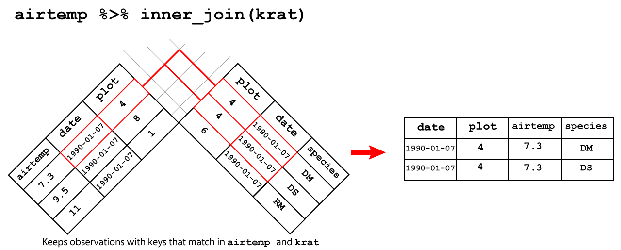
Figure 3.3: Inner join
## Joining, by = c("date", "plot")## # A tibble: 2 x 4
## date plot airtemp species
## <date> <dbl> <dbl> <chr>
## 1 1990-01-07 4 7.3 DM
## 2 1990-01-07 4 7.3 DS3.3.2.2 Left join
left_join(): keeps all the observations in the left hand table
An left join between airtemp and krat keeps all the observations in
airtemp and fills the missing observations in species with NA as shown
in Figure 3.4.
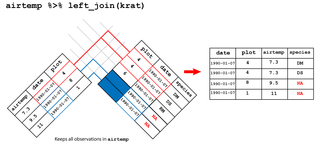
Figure 3.4: Left join
## Joining, by = c("date", "plot")## # A tibble: 4 x 4
## date plot airtemp species
## <date> <dbl> <dbl> <chr>
## 1 1990-01-07 4 7.3 DM
## 2 1990-01-07 4 7.3 DS
## 3 1990-01-07 8 9.5 <NA>
## 4 1990-01-07 1 11 <NA>3.3.2.3 Right join
right_join(): keeps all the observations in the right hand tables
An right join between airtemp and krat keeps all the observations in
krat and fills the missing observations in airtemp with NA as shown in
Figure 3.5.
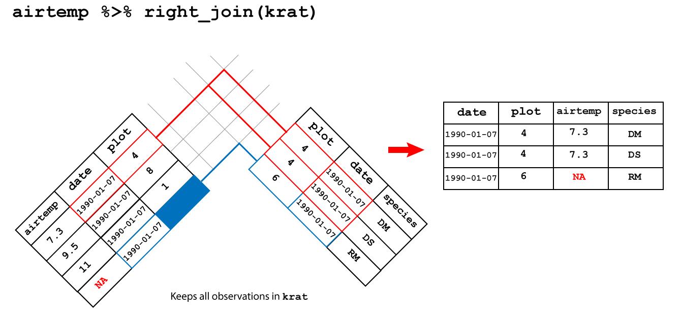
Figure 3.5: Right join
## Joining, by = c("date", "plot")## # A tibble: 3 x 4
## date plot airtemp species
## <date> <dbl> <dbl> <chr>
## 1 1990-01-07 4 7.3 DM
## 2 1990-01-07 4 7.3 DS
## 3 1990-01-07 6 NA RM3.3.2.4 Full join
full_join(): keeps all the observations in both tables
An full join between airtemp and krat keeps all the observations in
both tables and fills the missing observations in airtemp and species with NA as shown in
Figure 3.6.
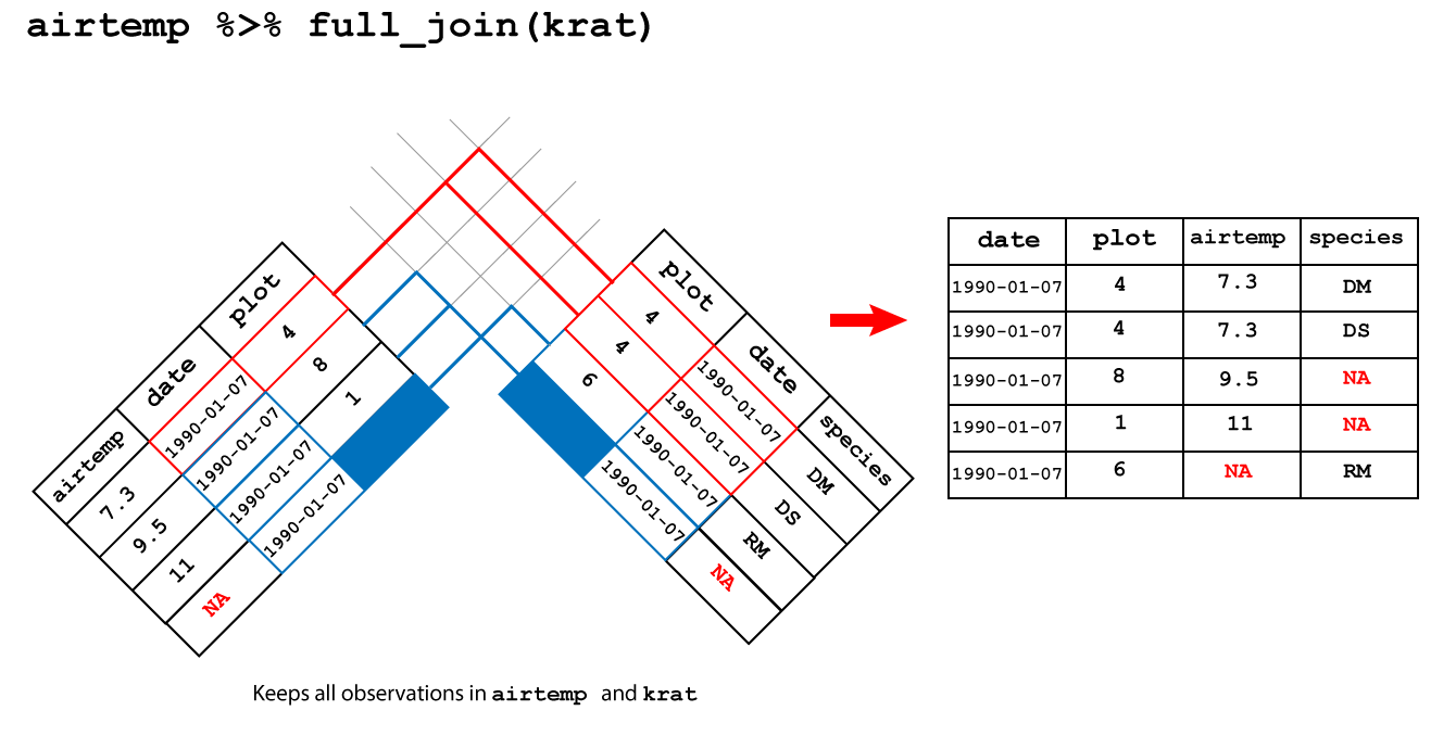
Figure 3.6: Full join
## Joining, by = c("date", "plot")## # A tibble: 5 x 4
## date plot airtemp species
## <date> <dbl> <dbl> <chr>
## 1 1990-01-07 4 7.3 DM
## 2 1990-01-07 4 7.3 DS
## 3 1990-01-07 8 9.5 <NA>
## 4 1990-01-07 1 11 <NA>
## 5 1990-01-07 6 NA RM3.3.3 Filtering joins
Filtering joins act like the filter function keeping only observations
that match the join without adding or removing columns.
semi_join() and anti_join()
3.3.3.1 Semi join
semi_join()keeps only the observations in the left hand table that have a match in the right hand table.
A semi-join between between airtemp and krat keeps only the observation
in airtemp that matches in krat as showin in Figure 3.7.
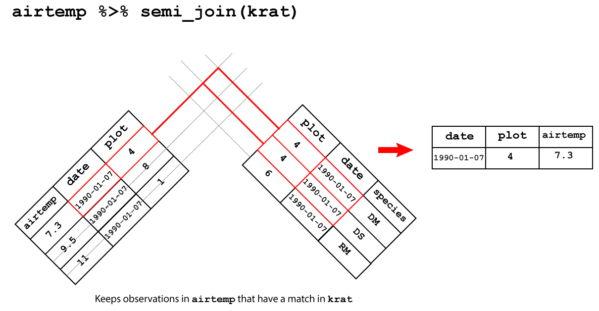
Figure 3.7: Semi join
## Joining, by = c("date", "plot")## # A tibble: 1 x 3
## date plot airtemp
## <date> <dbl> <dbl>
## 1 1990-01-07 4 7.33.3.3.2 Anti join
anti_join()drops the observations in the left hand table that have a match in the right hand table.
A anti-join between between airtemp and krat drops the observations
in airtemp that match in krat as shown in
Figure 3.8.
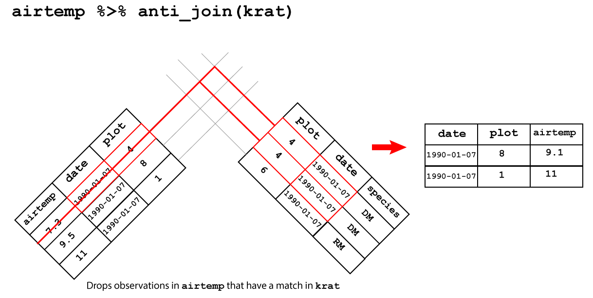
Figure 3.8: Anti join
## Joining, by = c("date", "plot")## # A tibble: 2 x 3
## date plot airtemp
## <date> <dbl> <dbl>
## 1 1990-01-07 8 9.5
## 2 1990-01-07 1 113.3.4 Set operations
These are joins corresponding with the
mathematical operation of intersection \(\cap\), union \(\cup\), and difference \(-\)
as shown in Figure 3.9. These are intersect(), union()
and setdiff().
See R4DS set operations for examples of usage.
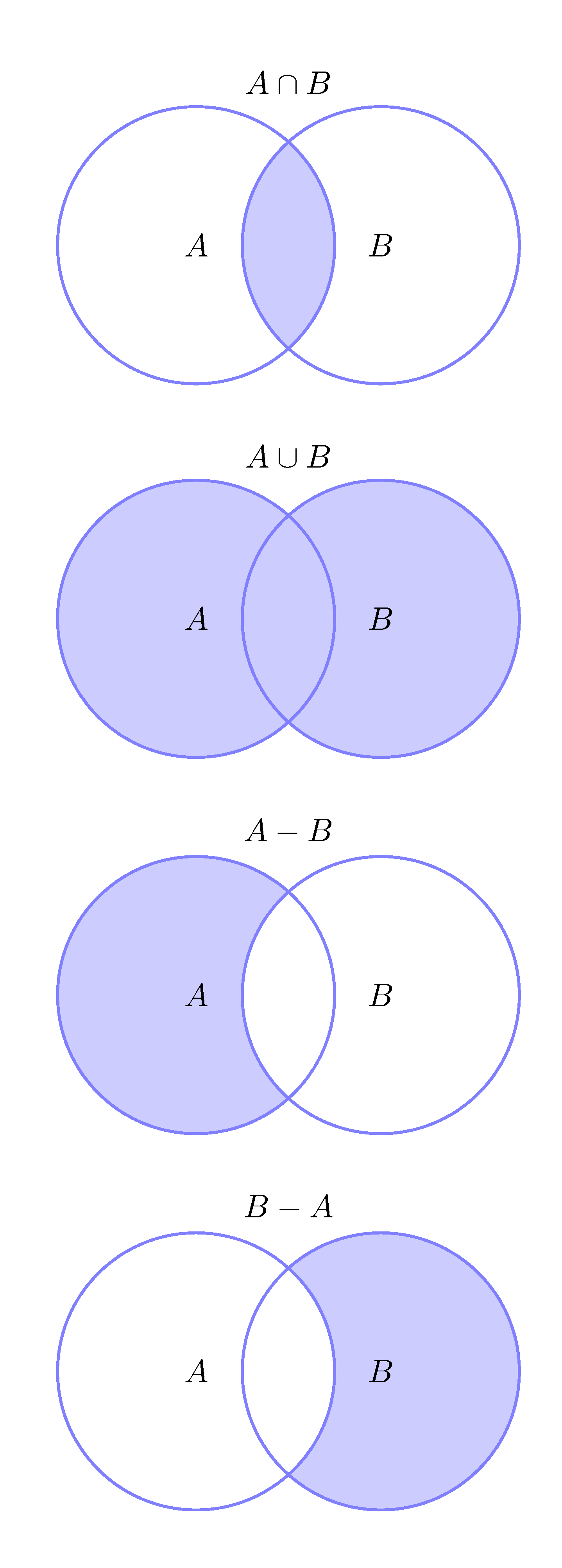
Figure 3.9: Set operations intersect(A,B), union(A,B) and setdiff(A,B).
3.3.5 Duplicate keys
If we have duplicate keys in each tables which aren’t used as part of the join, then
the join will create columns for both varaibles. For example, if we join airtemp
with krat only using plot as a key, but date is in both, we reuturn date.x and
date.y for airtemp and krat respecitively:
## # A tibble: 5 x 5
##   date.x      plot airtemp date.y     species
##   <date>     <dbl>   <dbl> <date>     <chr>
## 1 1990-01-07     4     7.3 1990-01-07 DM
## 2 1990-01-07     4     7.3 1990-01-07 DS
## 3 1990-01-07     8     9.5 NA         <NA>
## 4 1990-01-07     1    11   NA         <NA>
## 5 NA             6    NA   1990-01-07 RM
3.3.6 Binding rows and columns
We can also join tables by binding rows or columns. Binding rows is useful when we have tables with different sets of observations for the same variables, such as when we have multiple replicates of an experiment. Binding columns can be done when we want to add a column from one table that corresponds with the observations in another.
See dplyr bind :
“When row-binding, columns are matched by name, and any missing columns will be filled with NA.”
When column-binding, rows are matched by position, so all data frames must have the same number of rows."
These functions are bind_rows and bind_cols.