5 Functions, excel and combining plots
This extra chapter introduces:
- Using pseudocode before writing your actual code
- Writing your own functions
- Working with excel spreadsheets
- Using
patchworkto combine plots
5.1 Pseudocode
Pseudocode is the idea that we write down the steps of what we want to do in plain language to help us think about the actual code syntax we need to write.
For example, with the Portal surveys data we had a table with observations for several plot types in, but we were only interested in the control and long-term kangaroo rat exclosure plots.
So that step in pseudocode is:
I want make a table with only the observations for control and long-term kangaroo rat exclosure from the survey data.
In steps:
- Pipe the
surveystable to the filter function. - Pass arguments to the filter function to filter for observations equal to the control plot type or observations equal to the long-term kangaroo rat exclosure plot type.
In R code this becomes:
## # A tibble: 20,729 x 13
##    record_id month   day  year plot_id species_id sex   hindfoot_length weight
##        <dbl> <dbl> <dbl> <dbl>   <dbl> <chr>      <chr>           <dbl>  <dbl>
##  1         1     7    16  1977       2 NL         M                  32     NA
##  2        72     8    19  1977       2 NL         M                  31     NA
##  3       224     9    13  1977       2 NL         <NA>               NA     NA
##  4       266    10    16  1977       2 NL         <NA>               NA     NA
##  5       349    11    12  1977       2 NL         <NA>               NA     NA
##  6       363    11    12  1977       2 NL         <NA>               NA     NA
##  7       435    12    10  1977       2 NL         <NA>               NA     NA
##  8       506     1     8  1978       2 NL         <NA>               NA     NA
##  9       588     2    18  1978       2 NL         M                  NA    218
## 10       661     3    11  1978       2 NL         <NA>               NA     NA
## # … with 20,719 more rows, and 4 more variables: genus <chr>, species <chr>,
## #   taxa <chr>, plot_type <chr>
It can take a while and some research to figure out how to translate pseudocode to R code, and there is often more than one way to acheive the same result, but the point of the pseudocode is that it forces us to be specific about what we want to do. You may even have to re-write the pseudocode several times or talk to someone else to refine the question and then steps required to answer it.
The same approach can be used in many other areas of problem solving, such as experimental design.
5.2 Functions
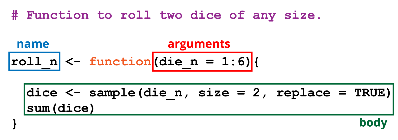
Functions are objects, and comprise of three parts:
- Name: short, but meaningful is advised
- Arguments: the inputs to the function
- Body: the code that does something with the arguments to create an output.
The body will generally use other functions, strung together to create our new function.
Let’s illustrate this by creating a function to simulate rolling a pair of dice, as per Hands on Programming with R

First we write some code that will become our function:
# Assign the numbers to a die
die <- 1:6
# Sample the die numbers twice
dice <- sample(die, size = 2, replace = TRUE)
# Add them together
sum(dice)
## [1] 4Now we put those elements as the body of a function, and assign it to a function
called roll with no arguments:
# Roll two dice function
roll <- function(){
  die <- 1:6
  dice <- sample(die, size = 2, replace = TRUE)
  sum(dice)
}
What about doing this for a die of any number of sides?

We remove the die object from the body of the function and turn it into an
argument that can take a sequence of integer values. Here we provide a default
of 1 to 6. It’s good practice to supply a default argument.
# Roll two dice of any size
roll_n <- function(die = 1:6) {
  dice <- sample(die, size = 2, replace = TRUE)
  sum(dice)
}
5.3 Working with Excel spreadsheets
5.3.1 Gapminder
The Gapminder Foundation:
The mission of Gapminder Foundation is to fight devastating ignorance with a fact-based worldview that everyone can understand.
For example, the famously created a bubble chart of the life expectancy vs. income around the world.
All sorts of data is available on their website and can be downloaded in various formats. Here we have a set of data for income, and life expectancy in countries around the world recorded between 1952 and 2007. (This version of gapminder data originated from Tidyverse Booster, Hadley Wickham.)
# Download the gapminder data
download.file("https://github.com/ab604/ab604.github.io/raw/master/docs/gapminder.zip",
              destfile = "gapminder.zip")

# Unzip the the gapminder data
unzip("gapminder.zip")
There should now be a gapminder directory in your working directory containing
a folder of csv files and excel files. These contain the same data, but split in
various ways: by country, by year or by continent.
We’re going to work with the excel data, where the data is split across multiple sheets in the same file.
5.3.2 readxl package
We’ll be using tidyverse package readxl for importing the excel data. Some of
the notes below are based on a tutorial by Karlijn Willems
The basic syntax is similar to read_csv or read_tsv from the readr package
where you pass the file path and name as a character vector to the read_excel function.
The default is to read the first sheet in the workbook. If your workbook has
multiple sheets you can open and list the sheet names with the excel_sheets function.
Individual sheets must be read as individual tables.
For example, lets look at the sheets in gapminder-country.xlsx :
##   [1] "Afghanistan"              "Albania"
##   [3] "Algeria"                  "Angola"
##   [5] "Argentina"                "Australia"
##   [7] "Austria"                  "Bahrain"
##   [9] "Bangladesh"               "Belgium"
##  [11] "Benin"                    "Bolivia"
##  [13] "Bosnia and Herzegovina"   "Botswana"
##  [15] "Brazil"                   "Bulgaria"
##  [17] "Burkina Faso"             "Burundi"
##  [19] "Cambodia"                 "Cameroon"
##  [21] "Canada"                   "Central African Republic"
##  [23] "Chad"                     "Chile"
##  [25] "China"                    "Colombia"
##  [27] "Comoros"                  "Congo, Dem. Rep."
##  [29] "Congo, Rep."              "Costa Rica"
##  [31] "Cote d'Ivoire"            "Croatia"
##  [33] "Cuba"                     "Czech Republic"
##  [35] "Denmark"                  "Djibouti"
##  [37] "Dominican Republic"       "Ecuador"
##  [39] "Egypt"                    "El Salvador"
##  [41] "Equatorial Guinea"        "Eritrea"
##  [43] "Ethiopia"                 "Finland"
##  [45] "France"                   "Gabon"
##  [47] "Gambia"                   "Germany"
##  [49] "Ghana"                    "Greece"
##  [51] "Guatemala"                "Guinea"
##  [53] "Guinea-Bissau"            "Haiti"
##  [55] "Honduras"                 "Hong Kong, China"
##  [57] "Hungary"                  "Iceland"
##  [59] "India"                    "Indonesia"
##  [61] "Iran"                     "Iraq"
##  [63] "Ireland"                  "Israel"
##  [65] "Italy"                    "Jamaica"
##  [67] "Japan"                    "Jordan"
##  [69] "Kenya"                    "Korea, Dem. Rep."
##  [71] "Korea, Rep."              "Kuwait"
##  [73] "Lebanon"                  "Lesotho"
##  [75] "Liberia"                  "Libya"
##  [77] "Madagascar"               "Malawi"
##  [79] "Malaysia"                 "Mali"
##  [81] "Mauritania"               "Mauritius"
##  [83] "Mexico"                   "Mongolia"
##  [85] "Montenegro"               "Morocco"
##  [87] "Mozambique"               "Myanmar"
##  [89] "Namibia"                  "Nepal"
##  [91] "Netherlands"              "New Zealand"
##  [93] "Nicaragua"                "Niger"
##  [95] "Nigeria"                  "Norway"
##  [97] "Oman"                     "Pakistan"
##  [99] "Panama"                   "Paraguay"
## [101] "Peru"                     "Philippines"
## [103] "Poland"                   "Portugal"
## [105] "Puerto Rico"              "Reunion"
## [107] "Romania"                  "Rwanda"
## [109] "Sao Tome and Principe"    "Saudi Arabia"
## [111] "Senegal"                  "Serbia"
## [113] "Sierra Leone"             "Singapore"
## [115] "Slovak Republic"          "Slovenia"
## [117] "Somalia"                  "South Africa"
## [119] "Spain"                    "Sri Lanka"
## [121] "Sudan"                    "Swaziland"
## [123] "Sweden"                   "Switzerland"
## [125] "Syria"                    "Taiwan"
## [127] "Tanzania"                 "Thailand"
## [129] "Togo"                     "Trinidad and Tobago"
## [131] "Tunisia"                  "Turkey"
## [133] "Uganda"                   "United Kingdom"
## [135] "United States"            "Uruguay"
## [137] "Venezuela"                "Vietnam"
## [139] "West Bank and Gaza"       "Yemen, Rep."
## [141] "Zambia"                   "Zimbabwe"
And then load the United Kingdom sheet and assign it to uk_dat:
References to sheet names are character vectors and therefore do require quotes.
Sheet indexing starts at 1, so alternatively, you could load in the 134th sheet for the UK with the following code:
In the read_excel function, if the col_names argument is left to its default value of TRUE, you will import the first line of the worksheet as the header names.
Alternatively, if you wish to skip using header specified column-names and instead “number columns sequentially from ...1 to ...N”, then set this argument to false: i.e. col_names = FALSE
Likewise you can override the default data types assigned by read_excel using
the col_types argument.
For example, if you wanted to set a three column excel sheet to contain the data
as dates in the first column, characters in the second, and numeric values in the third,
you would need the following lines of code:
For the final of the most useful additional arguments available in read_excel,
if you wish to skip rows before setting column names, there is the skip argument.
For example, if the spreadsheet had blank rows or other information in the first
five rows, and the column headers in the sixth row, using skip = 5 will read
the spreadsheet correctly.
5.4 Map functions
Let’s think about how we might read a number of excel sheets into a single data frame. We met map functions in Chapter 3.
Map functions allow us to iterate an operation:
The map functions transform their input by applying a function to each element and returning a vector the same length as the input.
There are lots of examples of using them in R4DS map functions.
Let’s state the problem in pseudocode terms. The gapminder year spreadsheet contains a sheet for every year between 1952 and 2007 recording life expectancy, population, country and continent:
We’d like to read all the sheets of the gapminder year spreadsheet into a single table that adds a column to indicate the year of the observations.
In steps:
- Create an object with the path to the spreadsheet
- Create an object with the names of the individual sheetss in the spreadsheet
- Read every sheet into a single data frame, creating a year variable from the sheet name
# Get the path to the gapminder year spreadsheet
path <- "gapminder/excel/gapminder-year.xlsx"
# Create a named character vector using the sheet names
sheets <- set_names(excel_sheets(path))

# Check code for the first sheet
read_excel(path, sheet = sheets[[1]])

# Now map all sheets to a single data frame and create a year variable from
# the sheet name
map_dfr(sheets, ~ read_excel(path, sheet = .x), .id = "year")
Now try the same approach to create the gapminder data using the gapminder/excel/gapminder-country.xlsx
spreadsheet combining all the invidual country sheets into a single table:
# replicate for excel/gapminder-country.xlsx to create gapminder data
path <- "gapminder/excel/gapminder-country.xlsx"
# Create a named character vector using the sheet names
sheets <- set_names(excel_sheets(path))

# Check code for first sheet
read_excel(path, sheet = sheets[[1]])
# Now map all sheets to a single data frame and create a country variable from
# the sheet name
gapminder <- map_dfr(sheets, ~ read_excel(path, sheet = .x), .id = "country")
Here the map function takes each value in sheets as passes it as .x to the
sheet argument of read_excel and also it as the value for a new variable country
created by the .id argument so that each observation in the new combined table
corresponds with the country sheet from which it derived.
Let’s look at the gapminder table we created for all the countries.
## Observations: 1,704
## Variables: 6
## $ country   <chr> "Afghanistan", "Afghanistan", "Afghanistan", "Afghanistan",…
## $ year      <dbl> 1952, 1957, 1962, 1967, 1972, 1977, 1982, 1987, 1992, 1997,…
## $ pop       <dbl> 8425333, 9240934, 10267083, 11537966, 13079460, 14880372, 1…
## $ continent <chr> "Asia", "Asia", "Asia", "Asia", "Asia", "Asia", "Asia", "As…
## $ lifeExp   <dbl> 28.801, 30.332, 31.997, 34.020, 36.088, 38.438, 39.854, 40.…
## $ gdpPercap <dbl> 779.4453, 820.8530, 853.1007, 836.1971, 739.9811, 786.1134,…
5.4.1 Lollipop plot function
Imagine we wanted to create a plot showing the population in each country, for any continent, for any of the years when the gapminder survey was carried out. Rather writing the code for each plot every time, we could write a function where we can pass the continent and year as arguments.
In the code below we create a lollipop plot, which is a sort of barplot, using two geoms, point and segment.
Step wise the body of the function does the following:
- Mutate the data to create a new
cpopfactor variable of each country ordered according to the population variable. - The data is then filtered for observations corresponding to the continent and year arguments.
- Call
ggplotwith aestheticsx = cpopandy = pop. - Add a point geom.
- Add a segment for the lollipop stick going from each
cpopon the x-axis, starting at 0 on the y-axis to the thepopvalue. - Turn the plot 90 degrees
- Change the axis labels
- Hide the legend
plot_lollipop <-
        function(dat = gapminder,
                 cnt = "Europe",
                 yr = 1997) {
                dat %>%
                        mutate(cpop = fct_reorder(country, pop)) %>%
                        filter(continent == cnt & year == yr) %>%
                        ggplot(aes(x = cpop, y = pop)) +
                        geom_point() +
                        geom_segment(aes(
                                xend = cpop,
                                y = 0,
                                yend = pop
                        )) +
                        coord_flip() +
                        labs(x = "Population",
                             y = "Country") +
                        theme(legend.position = "")
        }

# Use the function with default arguments
plot_lollipop()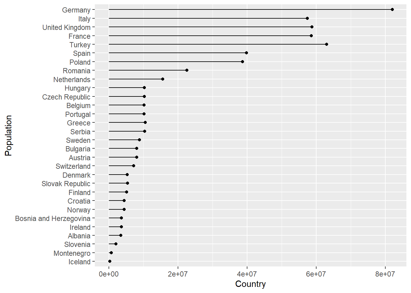
Just to illustrate how this can be extended further using a map function again to iterate through each continent. See R4DS on iteration.
This shows how functions can automate a task with a little bit of upfront effort.
Here we pass each value of con_names to our plot_lollipop function cnt argument
as .x in the same way we did for sheet = in when using map_dfr with read_excel.
# Create a vector of continent names
con_names <- gapminder %>% select(continent) %>% distinct() %>% pull()

# Plot using map function as before
map(con_names, ~ plot_lollipop(gapminder, .x, 1997))
## [[1]]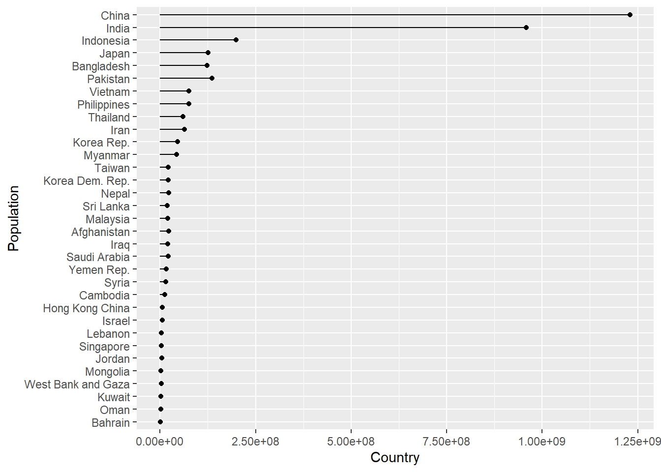
##
## [[2]]
##
## [[3]]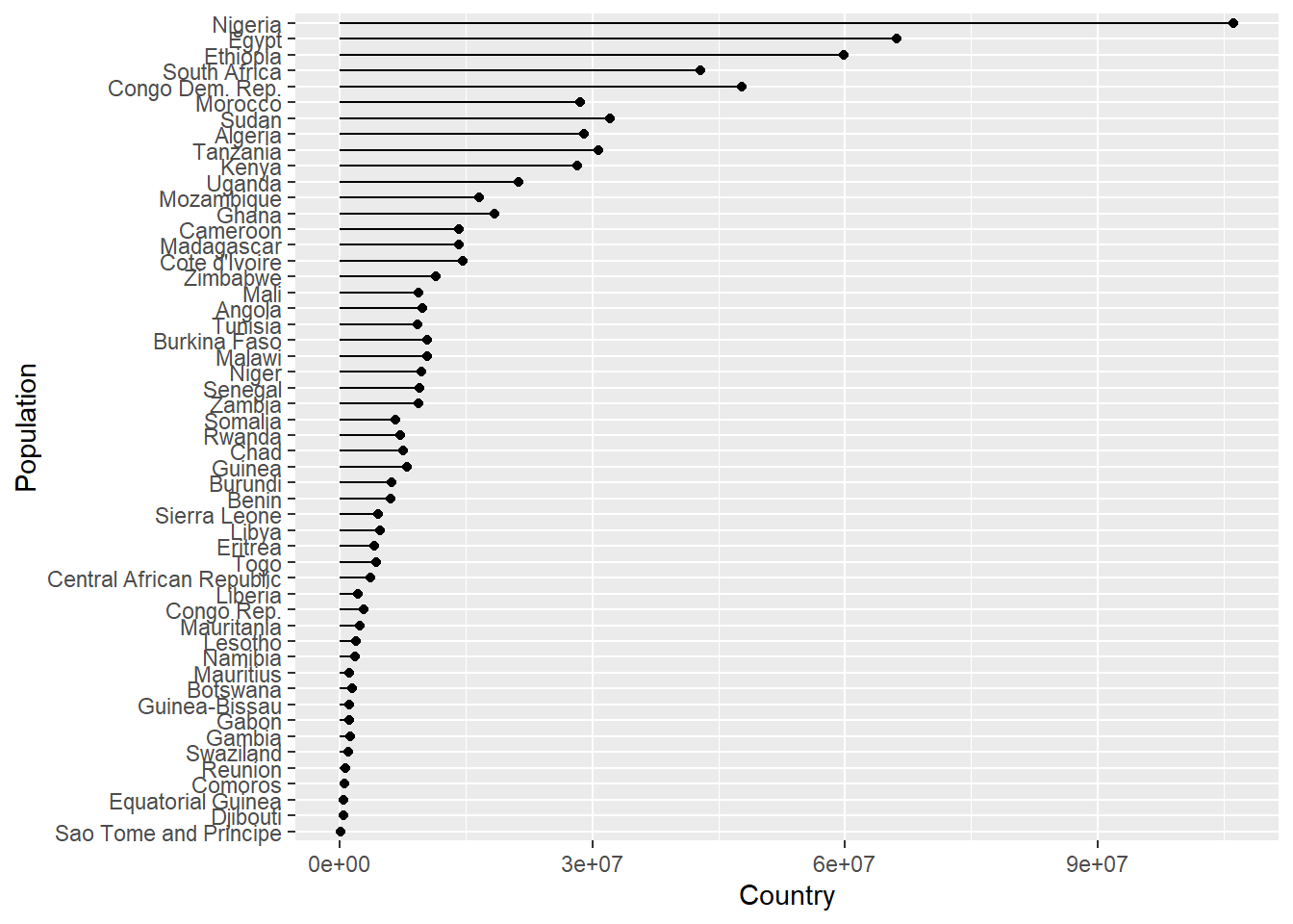
##
## [[4]]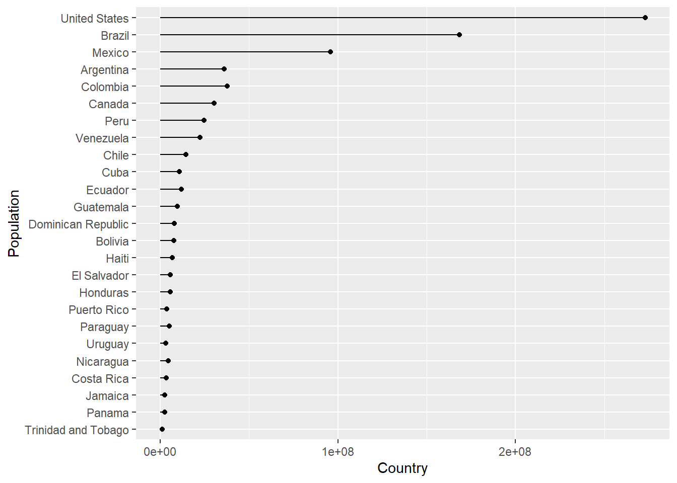
##
## [[5]]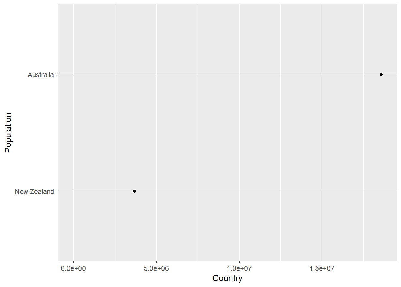
5.5 Combining plots with patchwork
See the patchwork website for lots more guidance.
5.5.1 Create four gapminder plots
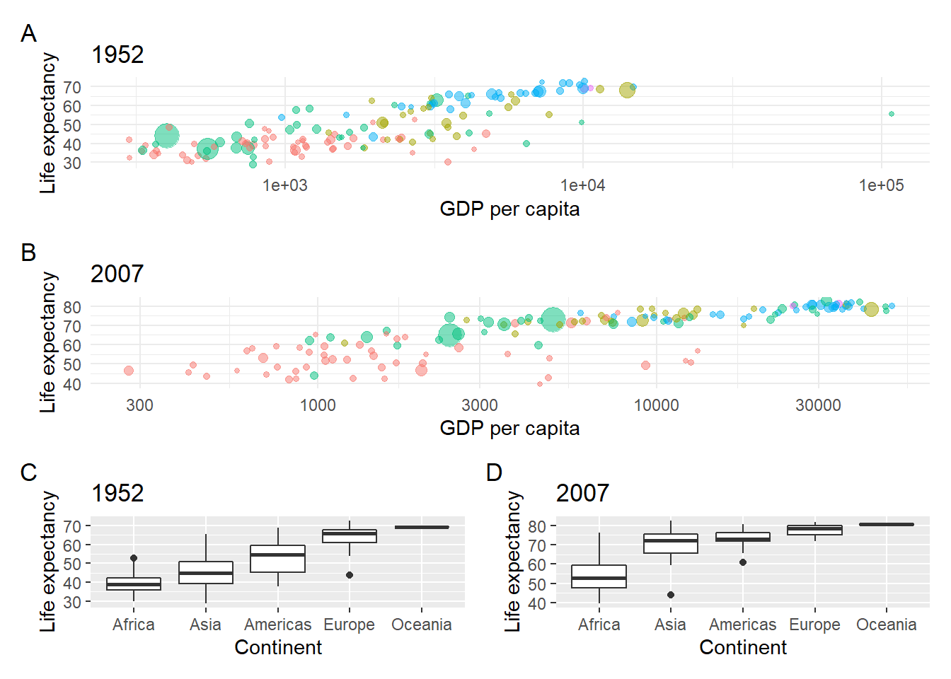
Let’s create four plots from the gapminder data:
- A bubble plot for life expectancy vs. gdp per capita in 1952 2 A bubble plot for life expectancy vs. gdp per capita in 2007
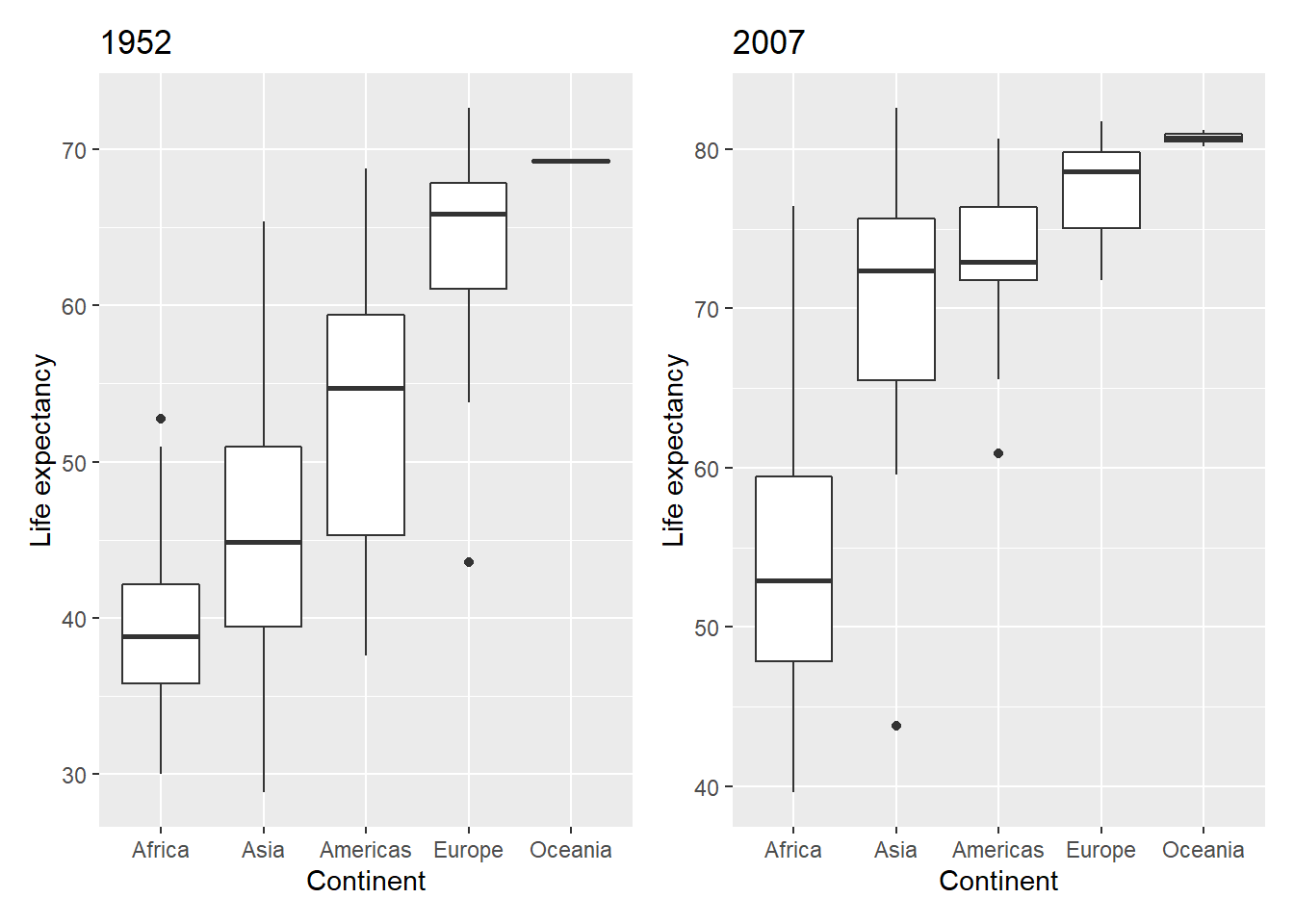
- A life expectancy boxplot for each continent in 1952
- A life expectancy boxplot for each continent in 2007
# Life expectancy bubble plot for 2007
bubble_1952 <- gapminder %>% filter(year == 1952) %>%
  ggplot(aes(x = gdpPercap,y = lifeExp, colour = continent, size = pop)) +
  geom_point(alpha = 0.5) +
  scale_x_log10() +
  theme_minimal() +
        labs(x = "GDP per capita", y = "Life expectancy") +
                        theme(legend.position = "") +
  ggtitle("1952")


# Life expectancy bubble plot for 2007
bubble_2007 <- gapminder %>% filter(year == 2007) %>%
  ggplot(aes(x = gdpPercap,y = lifeExp, colour = continent, size = pop)) +
  geom_point(alpha = 0.5) +
  scale_x_log10() +
  theme_minimal() +
        labs(x = "GDP per capita", y = "Life expectancy") +
                        theme(legend.position = "") +
  ggtitle("2007")

# Life expectancy boxplot for 1952
box_1952 <- gapminder %>%
  filter(year == 1952) %>%
  ggplot(aes(x = fct_reorder(continent,lifeExp),
             y = lifeExp)) +
  geom_boxplot() +
        labs(x = "Continent", y = "Life expectancy") +
  ggtitle("1952")

# Life expectancy boxplot for 2007
box_2007 <- gapminder %>%
  filter(year == 2007) %>%
  ggplot(aes(x = fct_reorder(continent,lifeExp),
             y = lifeExp)) +
  geom_boxplot() +
        labs(x = "Continent", y = "Life expectancy") +
  ggtitle("2007")
The basic syntax is + to add a plot. Let’s plot the two boxplots.
Use brackets () to group plots and forwardslash / to create a new row.
Now plot the bubble plots, each one on its own row, and group the boxplots onto
a single row:
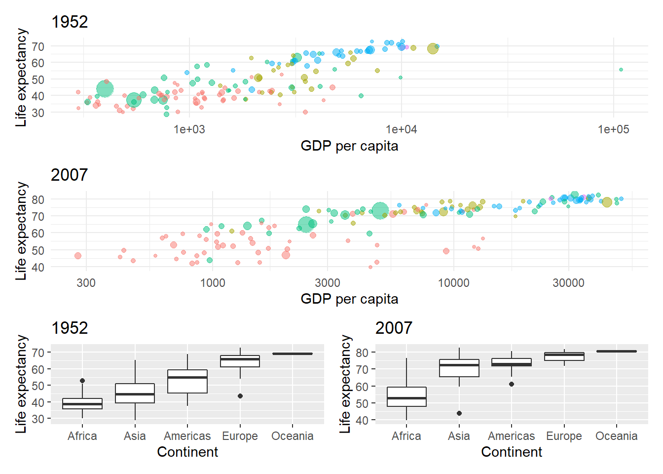
And plot_annotation(tag_levels = "A") with tag labels to add plot labels.