2  Markup Languages

Summary

This chapter can be skipped if you just want to learn about R. It introduces markup languages, confusingly called markdown, that encode text and documents such as the one you are reading.

The relevance here is two-fold:

1. Languages such as R can be integrated with markup languages to do what is called literate programming where one writes code and text in the same document. As opposed to writing code script(s) and report(s) separately. The code and text are evaluated separately, but outputted together.
2. Markup languages work with the universal document converter Pandoc, hence working in markdown means one can easily produce outputs in Word, pdf, html etc. all from the same input document.

2.1 What is markup?

Wikipedia has detailed pages on the history of typesetting pre and post the invention of computing. For example, the Wikipedia page on letter case describes how capital letters were often kept in the upper case of the drawers that contained the letters used in the printing press. Hence upper-case meaning capital in typesetting.

Much of this typography jargon naturally got carried over when computers came along, and marking up is both a digital and analogue term.

In the analogue sense markup is usually an instruction or comment to the author for revisions.

In the digital sense marking up is syntax on how to format or structure the text e.g. a heading, line break, bold or italic when it is rendered. Here you are reading Quarto markdown (Section 2.4.4) that has been rendered as a html book.

Again the Wikipedia markup languages page is great if you want the full details.

MS Word documents are markup language files in a XML format.

As an aside, it’s often possible to make sense of computing jargon if you can trace the analogue history in the relevant domain. Such as the term layers in computer graphics deriving from layers of paper used in pre-computing design.

2.2 What is markdown?

So why markdown?

Readability is the short answer, but again a longer better answer is on the Markdown Wikipedia page and the Markdown project page.

Markdown was created to be human readable and easy to write, as compared with heavier markup languages such as html or xml. And its growing popularity since 2004 and off-shoot flavours of markdown suggest it has been successful.

Below is are examples of markdown source code and outputs, where # marks up a first level header ## marks up the second level header, and ### marks up the third level header. Bullet points are marked-up with + or - .

Markdown Syntax	Output
# A First Level Header	A First Level Header
## A Second Level Header	A Second Level Header
### A Third Level Header	A Third Level Header
This is a regular paragraph.	This is a regular paragraph.
- A bullet point	A bullet point
	Caption

The heading to this chapter (Chapter 2) is a first level heading and this section has a second level heading (Section 2.2). The style e.g. font and colour and output (a html book) is controlled by another document, a configuration file.

2.3 Literate programming

Literate programming is a concept created by Donald Knuth of mixing code and prose in the same document. The resulting document can be tangled to run the code and weaved to created a human readable document.

In practice this looks like chunks of prose such as the one you are reading, mixed with chunks of code such as the one below. The R code chunk calls the in-built R constant called letters that contains the 26 characters of the English alphabet. Code chunks can be set in different ways, to be visible or hidden, to evaluate the code or not, and so on. Here it is set to evaluate and print the output below.

letters

 [1] "a" "b" "c" "d" "e" "f" "g" "h" "i" "j" "k" "l" "m" "n" "o" "p" "q" "r" "s"
[20] "t" "u" "v" "w" "x" "y" "z"

Try LETTERS to see the diffence between letters and LETTERS.

Literate programming is a trade-off: it’s slow and verbose, but if written well, easier to understand and amend than traditional scripts. It suits certain tasks such as teaching and report writing. Another benefit is that it’s often possible to use the same input document to create different types of output. For example, the same R Markdown document can be published as webpage, a Word document, a PDF or a PowerPoint presentation with relatively little effort.

Literate programming can be done with a variety of languages, not just R, Examples of literate programming tools are Jupyter, VS Code, R Markdown and Quarto.

2.4 Different flavours of markdown

There are a number of different flavours of markdown. By flavour I mean they all have common aspects, but differences in functionality that have been added to each version. Here are some of the common flavours.

2.4.1 Markdown

The original markdown was created by John Gruber in 2004. It contained the syntax for text, images, tables etc. that we saw in Section 2.2. Details on the Markdown project page and in the markdown guide.

2.4.2 Github flavoured markdown

Github flavoured markdown is the variant used by the software development platform Github. Amongst other things, it added code block functionality such as the letters code block in Section 2.3 and strikethrough text.

2.4.3 R Markdown

Unsurpisingly, R Markdown is the version of markdown developed by the creators of RStudio and incorporates lots of functionality for combining markdown and R in the literate programming paradigm (Section 2.3).

You can find full details in the RStudio R Markdown documentation, the R Markdown book and the R Markdown cookbook.

If you’re interested in more technical detail of how document creation works in R Markdown here’s a Stack overflow post explaining the relationship between R markdown knitr and pandoc

2.4.4 Quarto markdown

Quarto is created by Posit, the same company that created RStudio. It builds upon R Markdown (Section 2.4.3), but is designed to be used with a variety of languages and tools for creating technical documents and reports. It simplifies some of the quirks of R Markdown and is supposedly easier for creating dynamic content such as dashboards.

As someone who started with LaTeX and then moved to R Markdown I’ve found it fairly straightfoward to change to Quarto and prefer it. Quarto comes bundled with RStudio from v2022.07.1, so we’ll use Quarto for our exercises.

There’s nothing wrong with sticking with R Markdown if you prefer it or feel it’s too much effort to change. But if you have exisiting R Markdown files and want to switch, you’ll find it’s fairly easy to convert them into Quarto markdown and may find long term benefits.

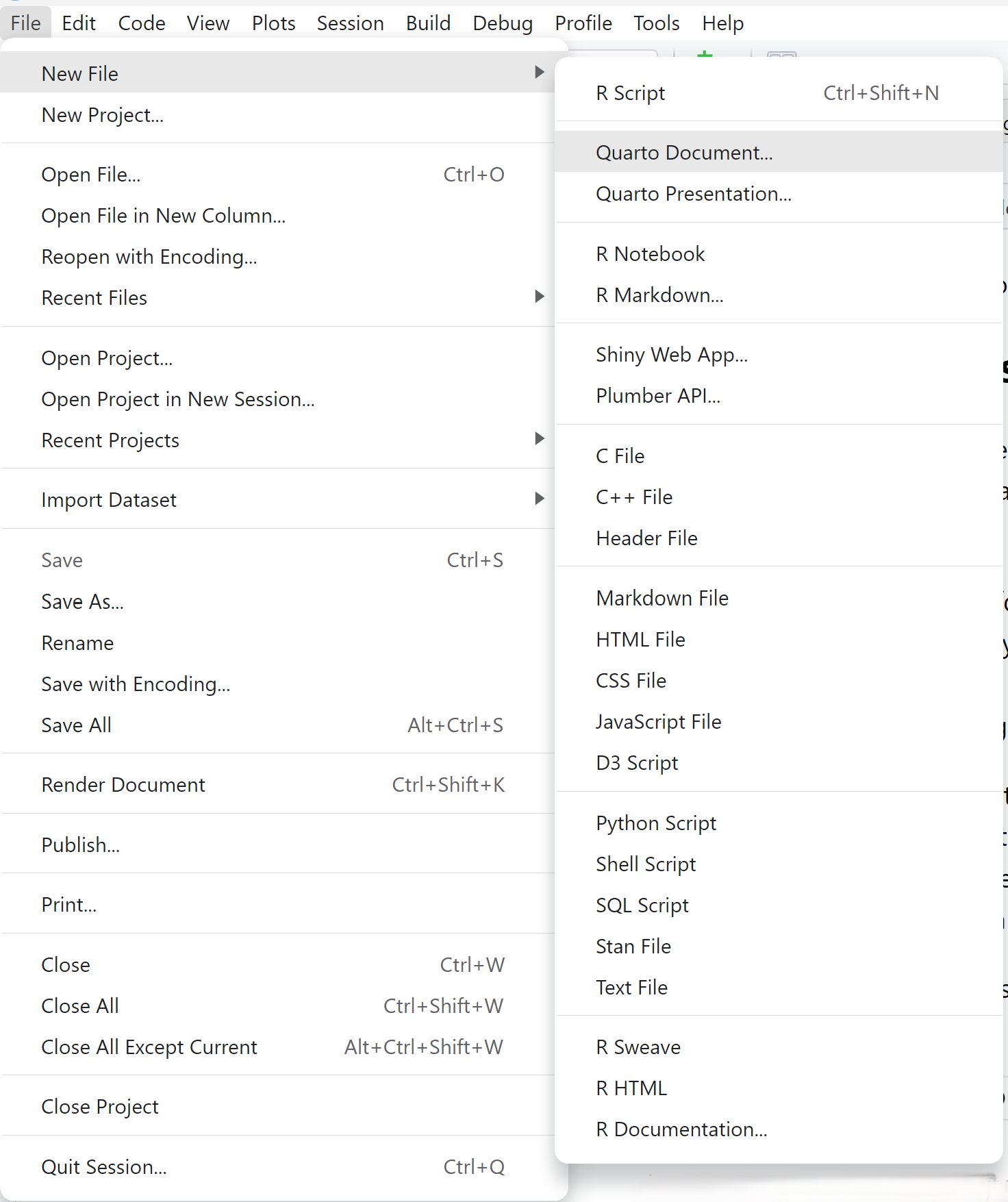
We can create a new document in R Studio from the File menu and then New File displays all the default file types available as shown in Figure 2.1. Here I highlighted a new Quarto Document.

Figure 2.1: Creating a new document in R Studio from the File menu

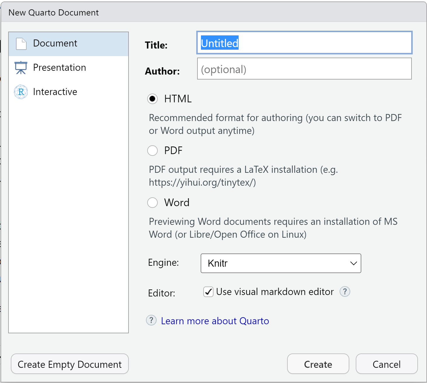
Selecting Quarto Document opens a dialogue box as shown in Figure 2.2, giving us the opportunity to set various features such as the default output document format or whether we want to create a document or presentation. This can all be changed later, so don’t worry if you change your mind.

Figure 2.2: Quarto Document dialogue box

2.5 Publishing outputs with Pandoc

Pandoc created in 2006 by John MacFarlane to convert one markup format to another, including HTML, XML, MS Word, PDF and all the various flavours of markdown.

As mentioned in Section 2.3, it can be quite time saving to write in a single markdown language and then create the various output documents as required for yourself or your collaborators.

RStudio comes bundled with pandoc so there’s no need to install it separately (unlesss you want to). Pandoc can be used independently of RStudio if you are willing to learn how to do data science at the command line. Perhaps a problem for another day?!