5  Data wrangling I

Summary

This chapter covers some common tasks for working with tabular data using the tidyverse packages dplyr and tidyr. The tasks are filtering for rows of interest, arranging the rows, selecting columns of interest, creating new columns, creating grouped summaries of the table, and re-shaping (aka pivoting) the table.

5.1 The pipe |>

The pipe operator |> allows you to combine operations by passing the output of an object or function to another. It will make more sense why this is a good thing once we start writing code, but you can think of it as a coding adverb such as then.

In the example below, the penguins data frame is piped to the count function from dplyr (Section 5.2) which has the species column as its argument.

Think of it as: Return the penguins table then count how many rows there are for each different penguin species.

Note that as I am not assigning the output to an object with <- (Section 3.9) the output is returned to the console.

Pipe style

The recommended pipe style is a space before a pipe and the pipe to be the last thing on a line, like so:

penguins |> 
  count(species)

# A tibble: 3 × 2
  species       n
  <fct>     <int>
1 Adelie      152
2 Chinstrap    68
3 Gentoo      124

This makes reading and adding new steps easier.

The pipe |> was added to R as of version 4.1.0 , you may see the %>% pipe from the magrittr package sometimes, but it’s simpler to use the native version. However, you may need to check the native pipe is enabled in the Options (Figure 5.1).

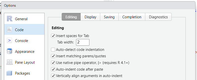
Figure 5.1: Setting the native pipe |> option in RStudio

The shortcut for the pipe operator is Ctl+Shift+M on Windows or Cmd+Shift+M on a Mac.

5.2 Introducing dplyr

dplyr “is a grammar of data manipulation”. Concretely, it’s a package of functions from the tidyverse that have been created for tasks that require manipulation of data stored in data frames Section 3.10.3.

As mentioned in Section 3.6, the grammar is the naming of the functions as verbs. Personally, I find this parallel between R code and human language makes things cognitively easier for me. I can describe what I want to do using natural language and translate it easily into tidyverse code.

Figure 5.2: Why is it called dplyr?

5.3 The four most common dplyr verbs

We’ll use the four most common verbs in dplyr to examine the Palmer Penguins data (Section 3.4.1).

5.3.1 Filter rows with filter()

To remind you, the penguins data frame has 344 rows (Section 3.4.1). Each row contains a set of observations contained in the columns for a single penguin from one of three species (Figure 3.6) living on one of three islands.

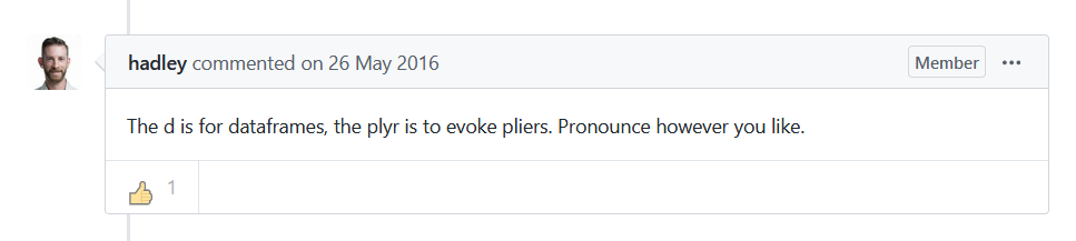
So if for example we wanted to filter the data frame for only the rows of penguins with a bills longer or equal to 50 mm, we would use the filter function as shown in Figure 5.3.

The function takes the penguins data frame object as the first argument. Either within the parentheses or via a pipe.

The second argument is the column (variable) we wish to filter on, in this case bill_length_mm and a logical expression (evaluates as TRUE or FALSE) that is the filter.

Here the expression is greater or equal to 50 >= 50.

So any row with a value in bill_length_mm greater or equal to 50 is TRUE and is retained and any row with a value less than 50 is FALSE and is discarded.

Figure 5.3: The dplyr filter function. The filter function returns rows from your data frame that satisfy your filter expression as TRUE. Here it will return all Palmer Penguins with a bill longer or equal to 50 mm. Here it shows how filter will return all Palmer Penguins with a bill longer or equal to 50 mm. The function can either be used by providing the penguins data.frame as the first argument to the function or by passing the penguins data frame via a pipe.

Here is the code, note that I’ve piped the output to the dplyr glimpse() function which prints a transposed summary of the filtered data frame contents to the console.

Instead of a table of 344 penguins, we’ve returned a data frame with the 57 penguins (rows) that have bills equal or longer than 50 mm, but we still have 8 columns (variables) as filter() only acts on the rows.

penguins |> 
  filter(bill_length_mm >= 50) |> 
  glimpse()

Rows: 57
Columns: 8
$ species           <fct> Gentoo, Gentoo, Gentoo, Gentoo, Gentoo, Gentoo, Gent…
$ island            <fct> Biscoe, Biscoe, Biscoe, Biscoe, Biscoe, Biscoe, Bisc…
$ bill_length_mm    <dbl> 50.0, 50.0, 50.2, 50.0, 59.6, 50.5, 50.5, 50.1, 50.4…
$ bill_depth_mm     <dbl> 16.3, 15.2, 14.3, 15.3, 17.0, 15.9, 15.9, 15.0, 15.3…
$ flipper_length_mm <int> 230, 218, 218, 220, 230, 222, 225, 225, 224, 231, 22…
$ body_mass_g       <int> 5700, 5700, 5700, 5550, 6050, 5550, 5400, 5000, 5550…
$ sex               <fct> male, male, male, male, male, male, male, male, male…
$ year              <int> 2007, 2007, 2007, 2007, 2007, 2008, 2008, 2008, 2008…

Filtering can be done using multiple columns and expressions. See the official filter documentation for more complex examples.

5.3.2 Arranging rows with arrange()

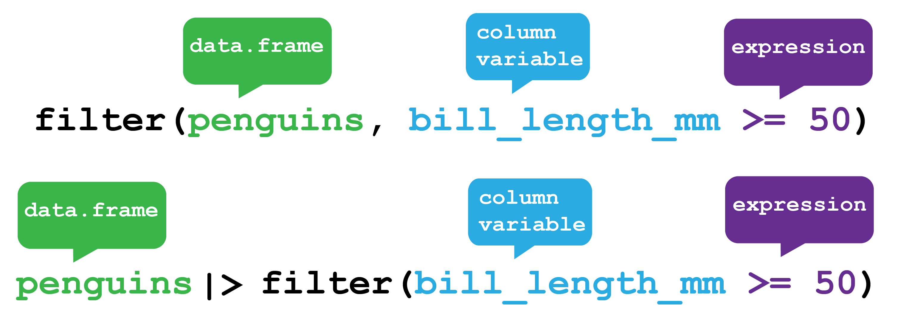
Another row verb is arrange() which as the name suggests arranges the rows according to column values (Figure 5.4).

Here I’ll pipe the penguins data frame to the base R head() function, which returns the first six rows by default. Again I am returning the output to the console.

I’ve formatted the output slightly here to highlight flipper_length_mm in red, so it may look a bit different to your output. We can see that row four is one of the two rows with missing values (indicated by NA) that we first encountered as a warning when we plotted this data (Section 3.11).

penguins |> 
  head() 

species	island	bill_length_mm	bill_depth_mm	flipper_length_mm	body_mass_g	sex	year
Adelie	Torgersen	391	187	181	3750	male	2007
Adelie	Torgersen	395	174	186	3800	female	2007
Adelie	Torgersen	403	180	195	3250	female	2007
Adelie	Torgersen	NA	NA	NA	NA	NA	2007
Adelie	Torgersen	367	193	193	3450	female	2007
Adelie	Torgersen	393	206	190	3650	male	2007

Next I add another line of code using arrange(flipper_length_mm) to sort the rows according to the values in this column. It defaults to ascending order.

penguins |> 
  arrange(flipper_length_mm) |> 
  head()

species	island	bill_length_mm	bill_depth_mm	flipper_length_mm	body_mass_g	sex	year
Adelie	Biscoe	379	186	172	3150	female	2007
Adelie	Biscoe	378	183	174	3400	female	2007
Adelie	Torgersen	402	170	176	3450	female	2009
Adelie	Dream	395	167	178	3250	female	2007
Adelie	Dream	372	181	178	3900	male	2007
Adelie	Dream	331	161	178	2900	female	2008

To arrange for descending order, I need to use the desc() function in combination with arrange() like so:

penguins |> 
  arrange(desc(flipper_length_mm)) |> 
  head()

species	island	bill_length_mm	bill_depth_mm	flipper_length_mm	body_mass_g	sex	year
Gentoo	Biscoe	543	157	231	5650	male	2008
Gentoo	Biscoe	500	163	230	5700	male	2007
Gentoo	Biscoe	596	170	230	6050	male	2007
Gentoo	Biscoe	498	168	230	5700	male	2008
Gentoo	Biscoe	486	160	230	5800	male	2008
Gentoo	Biscoe	521	170	230	5550	male	2009

Further guidance about arrange() from R4DS:

“If you provide more than one column name, each additional column will be used to break ties in the values of preceding columns… Missing values are always sorted at the end.”

Figure 5.4: The dplyr arrange function. The arrange function orders rows from your data frame according to column variables. Here it will order the Palmer Penguins data.frame according to their flipper length. The function can either be used by providing the penguins data.frame as the first argument to the function or by passing the penguins data.frame via a pipe.

5.3.3 Selecting columns with select()

Often your data contains variables you don’t need for the analysis you are performing, or you want to subset them to share with others. To select only the ones you need, or explore subsets of the variables, the select() verb enables you to keep only the columns of interest.

Figure 5.5 shows the use of select() to choose only the island and year columns, with or without the pipe.

Selecting the variables contained in the columns can be done in various ways. For example, by the column number, the variable name or by range. Check the help function ?select for more options.

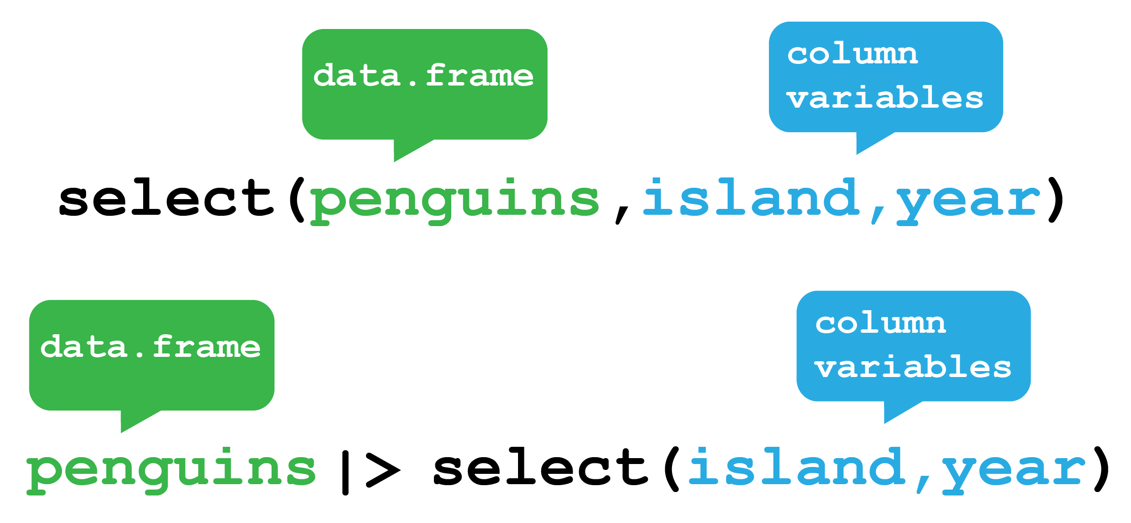
Figure 5.5: The dplyr select function. This function selects columns from your data frame. Here it will select the island and year columns from Palmer Penguins data.frame. The function can either be used by providing the penguins data.frame as the first argument to the function or by passing the penguins data.frame via a pipe.

Let’s do this a couple of ways, first reminding ourselves of what the columns are using glimpse(). I’ll continue with the piped approach.

penguins |> 
  glimpse()

Rows: 344
Columns: 8
$ species           <fct> Adelie, Adelie, Adelie, Adelie, Adelie, Adelie, Adel…
$ island            <fct> Torgersen, Torgersen, Torgersen, Torgersen, Torgerse…
$ bill_length_mm    <dbl> 39.1, 39.5, 40.3, NA, 36.7, 39.3, 38.9, 39.2, 34.1, …
$ bill_depth_mm     <dbl> 18.7, 17.4, 18.0, NA, 19.3, 20.6, 17.8, 19.6, 18.1, …
$ flipper_length_mm <int> 181, 186, 195, NA, 193, 190, 181, 195, 193, 190, 186…
$ body_mass_g       <int> 3750, 3800, 3250, NA, 3450, 3650, 3625, 4675, 3475, …
$ sex               <fct> male, female, female, NA, female, male, female, male…
$ year              <int> 2007, 2007, 2007, 2007, 2007, 2007, 2007, 2007, 2007…

So we can see the eight column names and that island is column 2 and year is column 8.

Let’s select by name:

penguins |> 
  select(island, year) |> 
  glimpse()

Rows: 344
Columns: 2
$ island <fct> Torgersen, Torgersen, Torgersen, Torgersen, Torgersen, Torgerse…
$ year   <int> 2007, 2007, 2007, 2007, 2007, 2007, 2007, 2007, 2007, 2007, 200…

By column number:

penguins |> 
  select(2,8) |> 
  glimpse()

Rows: 344
Columns: 2
$ island <fct> Torgersen, Torgersen, Torgersen, Torgersen, Torgersen, Torgerse…
$ year   <int> 2007, 2007, 2007, 2007, 2007, 2007, 2007, 2007, 2007, 2007, 200…

By negative selection using the minus sign - to exclude the columns we don’t want:

penguins |> 
  select(-species,-bill_length_mm, -bill_depth_mm,
         -flipper_length_mm,-body_mass_g, -sex) |> 
  glimpse()

Rows: 344
Columns: 2
$ island <fct> Torgersen, Torgersen, Torgersen, Torgersen, Torgersen, Torgerse…
$ year   <int> 2007, 2007, 2007, 2007, 2007, 2007, 2007, 2007, 2007, 2007, 200…

See the select documentation for other approaches for using select such as renaming columns, reordering the columns or picking variables with selection helper functions.

5.3.4 Creating new columns with mutate()

Another common task is to create a new variable or variables, often from existing data within the data frame. For this we use the mutate() verb. It follows the same syntax as for filter(), arrange() and select() in that the first argument is the dataset, and the subsequent arguments are the new variables we wish to create (Figure 5.6).

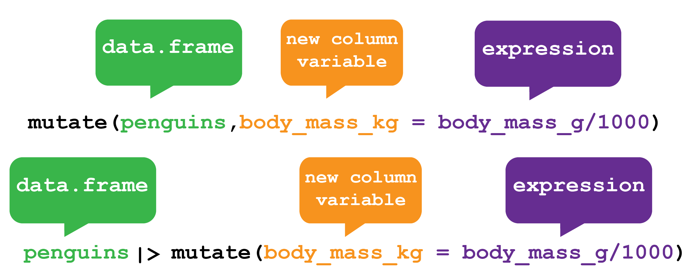
Figure 5.6: The dplyr mutate function. The mutate function creates new column variables in your data frame. Here mutate creates a new variable called body_mass_kg in the Palmer Penguins data.frame by dividing the values in the body_mass_g column by 1000 and storing the answer in new variable body_mass_kg. The function can either be used by providing the penguins data.frame as the first argument to the function or by passing the penguins data.frame via a pipe.

Here I’ll use the piped syntax again and glimpse() on the output to create a new variable for penguin body mass in kilograms called body_mass_kg from the existing body mass in grams variable by dividing by 1,000 using mutate().

I’m also going to use select() to select only the species, body_mass_g and new variable body_mass_kg and then head() to view the first six rows to make the output a bit easier to read.

penguins |> 
  mutate(body_mass_kg = body_mass_g/1000) |> 
  select(species, body_mass_g, body_mass_kg) |> 
  head()

species	island	body_mass_g	body_mass_kg
Adelie	Torgersen	3750	3.75
Adelie	Torgersen	3800	3.80
Adelie	Torgersen	3250	3.25
Adelie	Torgersen	NA	NA
Adelie	Torgersen	3450	3.45
Adelie	Torgersen	3650	3.65

5.4 Creating grouped summaries with dplyr

Another powerful feature of dplyr is it’s ability to summarise the entire dataset in a single row.

penguins |> 
  summarise(mean_mass_g = mean(body_mass_g, na.rm = TRUE))

# A tibble: 1 × 1
  mean_mass_g
        <dbl>
1       4202.

penguins |> 
  group_by(species) |> 
  summarise(mean_mass_g = mean(body_mass_g, na.rm = TRUE), 
            n_penguins = n())

# A tibble: 3 × 3
  species   mean_mass_g n_penguins
  <fct>           <dbl>      <int>
1 Adelie          3701.        152
2 Chinstrap       3733.         68
3 Gentoo          5076.        124

5.4.1 Using group_by() and summarise() together

Calculating the average bill length and depth for each species

pipe the penguins dataset into the group_by() function, which groups the data by the species variable. - We then use the summarise() function to calculate the average bill length and depth for each species using mean(). - The na.rm = TRUE argument is used to remove any missing values before calculating the means.

# Calculate the average bill length and depth for each species
penguins |>
  group_by(species) |>
  summarise(
    avg_bill_length = mean(bill_length_mm, na.rm = TRUE),
    avg_bill_depth = mean(bill_depth_mm, na.rm = TRUE)
  )

# A tibble: 3 × 3
  species   avg_bill_length avg_bill_depth
  <fct>               <dbl>          <dbl>
1 Adelie               38.8           18.3
2 Chinstrap            48.8           18.4
3 Gentoo               47.5           15.0

Count the number of penguins by island and sex. We start with the penguins dataset and pipe it into the group_by() function to group the data by both island and sex variables. As before, we then use the summarise() function along with n() to count the number of penguins in each group.

# Count the number of penguins by island and sex
penguins |>
  group_by(island, sex) |>
  summarise(mean_mass_g = mean(body_mass_g,na.rm = TRUE), 
            n_penguins = n())

# A tibble: 9 × 4
# Groups:   island [3]
  island    sex    mean_mass_g n_penguins
  <fct>     <fct>        <dbl>      <int>
1 Biscoe    female       4319.         80
2 Biscoe    male         5105.         83
3 Biscoe    <NA>         4588.          5
4 Dream     female       3446.         61
5 Dream     male         3987.         62
6 Dream     <NA>         2975           1
7 Torgersen female       3396.         24
8 Torgersen male         4035.         23
9 Torgersen <NA>         3681.          5

5.5 Pivots

Data can be untidy in different ways. One way might be that the values are in the variable names. Or perhaps the reverse is true and you’d like the values to be column names.

Reshaping a table is called pivoting. If one pivots a table that leads to increasing the number of rows one would use the tidyr package function pivot_longer() and if one pivots a table to increase the number of columns one would use pivot_wider() (Figure 5.7 and Figure 5.8).

Figure 5.7: pivot

Figure 5.8: pivot

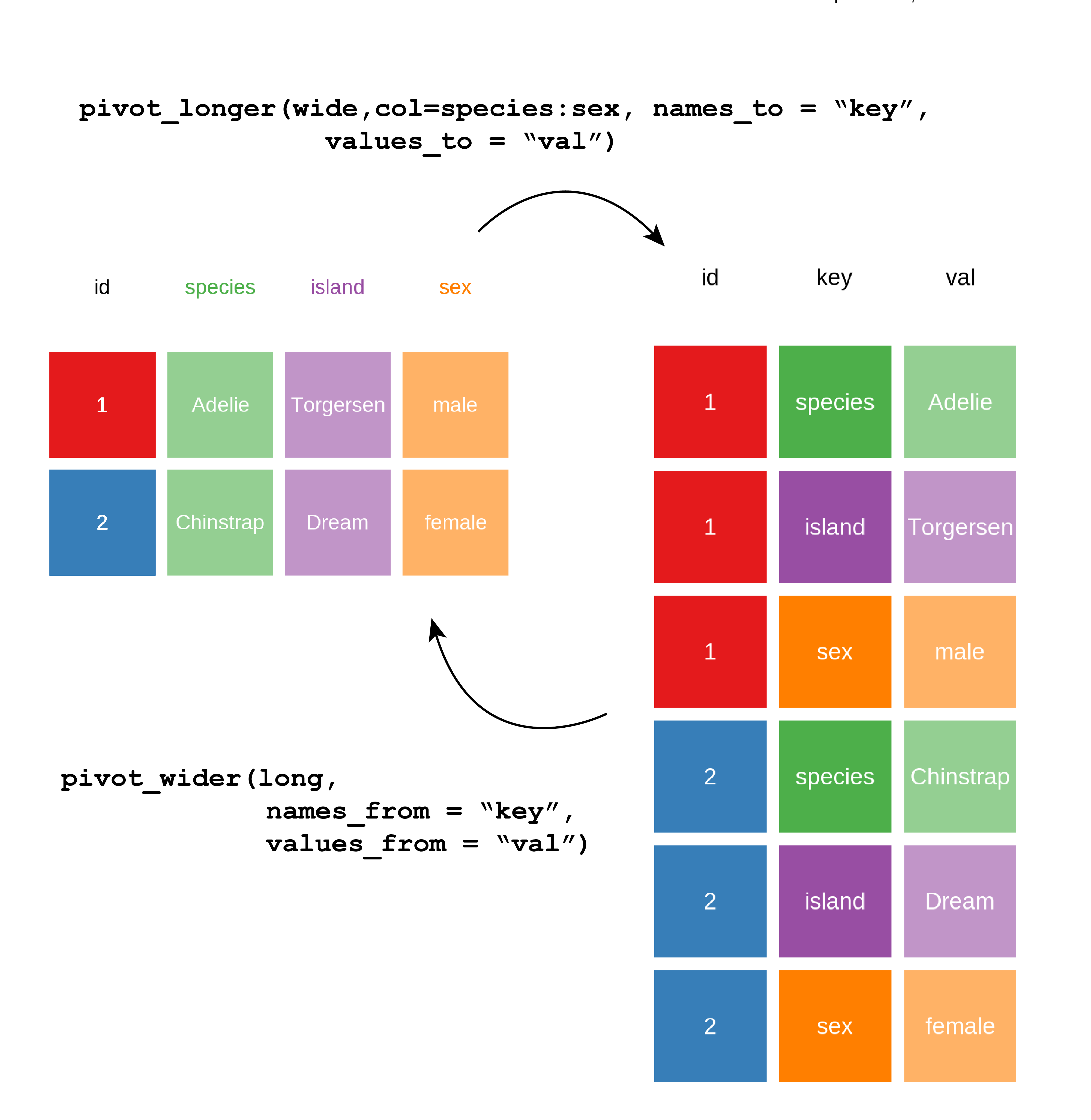
To demonstrate the pivot as in Figure 5.7 and Figure 5.8, we need a unique identifier for each row which I’ll create a variable called id using mutatae and the dplyr function row_number() which as you might guess, counts the row number and returns an integer.

We pivot longer by transforming column variable names, here: species , island and sex into values stored in a new variable that I’ve named key.

The existing values from those columns are placed in the cells of a new variable I’ve called val.

In this way the table gets longer as there are now three rows for the data about each penguin, hence the id column I created for each penguin has three repeating values, one for each row corresponding with the original columns.

# Pivot the data longer
penguins_long <- penguins |>
  # Add id column from row number to create a unique identifier
  mutate(id = row_number()) |> 
  select(species, island, sex, id) |> 
  pivot_longer(
    cols = species:sex,
    names_to = "key",
    values_to = "val"
  )

glimpse(penguins_long)  

Rows: 1,032
Columns: 3
$ id  <int> 1, 1, 1, 2, 2, 2, 3, 3, 3, 4, 4, 4, 5, 5, 5, 6, 6, 6, 7, 7, 7, 8, …
$ key <chr> "species", "island", "sex", "species", "island", "sex", "species",…
$ val <fct> Adelie, Torgersen, male, Adelie, Torgersen, female, Adelie, Torger…

To pivot from long to wide, we reverse the procedure by using values in key to create variable names for columns and populate the columns with the values from our val column.

This returns us to one row per penguin, with four columns.

# Pivot the data wider
penguins_wide <- penguins_long |> 
  pivot_wider(
    names_from = "key",
    values_from = "val"
  )

glimpse(penguins_wide)

Rows: 344
Columns: 4
$ id      <int> 1, 2, 3, 4, 5, 6, 7, 8, 9, 10, 11, 12, 13, 14, 15, 16, 17, 18,…
$ species <fct> Adelie, Adelie, Adelie, Adelie, Adelie, Adelie, Adelie, Adelie…
$ island  <fct> Torgersen, Torgersen, Torgersen, Torgersen, Torgersen, Torgers…
$ sex     <fct> male, female, female, NA, female, male, female, male, NA, NA, …

The trick with pivots is trying to understand which column variables you transform into as values to pivot longer. Or which values you want to become variables to pivot wider. If often takes a couple of attempts to get it right.