Chapter 3 Creating scripts and importing data
Our analysis is of an example data set of observations for 7702 proteins from cells in three control experiments and three treatment experiments. The observations are signal intensity measurements from the mass spectrometer. These intensities relate the concentration of protein observed in each experiment and under each condition.
We consider raw data as the data as we receive it. This doesn’t mean it hasn’t be processed in some way, it just means it hasn’t been processed by us. Generally speaking we don’t change the raw data file, what we do is import it and create an object in R which we then transform.
So let’s understand how to import some data.
3.1 Some definitions
- Importing means getting data into our R environment by creating an object that we can then manipulate. The raw data file remains unchanged.
- Inspecting means looking at the dataset to understand what it contains.
- Tidying refers to getting data into a consistent format that makes it easy to use in later steps.
3.1.1 Rectangular data and flat formats
Two further things to note:
Here we are only considering rectangular data, the sort that comes in rows and columns such as in a spreadsheet. Lots of our data types exist, such as images, but can also be handled by R. As mentioned in 3.5.1 genomic data in particular has led to a project called Bioconductor for the development of analysis tools primarily in R, many of which deal with non-rectangular data, but this is beyond the scope here.
Flat formats are files that only contain plain text, with each line representing a set of observations and the variables separated by delimiters such as tabs, commas or spaces. Therefore there aren’t multiple tables such as we’d get in an Excel file, or meta-data such as the colour highlighting of a cell in an Excel file. The advantages of flat files is that they can be opened and used by many different computing languages or programs. So unless there is a good reason not to use a flat format, and there are good reasons, they are the best way to store data in many situations.
3.2 Using scripts
Using the console is useful, but as we build up a workflow, that is to say, writing code to:
- load packages
- load data
- explore the data
- and output some results
Then it’s much more useful to contain this in a script: a document of our code.
Why? When we write and save our code in scripts, we can re-use it, share it or edit it. But most importantly a script is a record.
Cmd/Ctrl + Shift + N will open a new script file up and you should see something like Figure 3.1 with the script editor pane open:
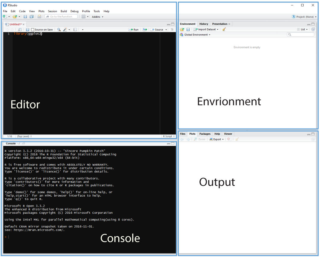
Figure 3.1: Rstudio with the script editor pane open.
3.3 Running code
We can run a highlighted portion of code in your script if you click the Run button at the top of the scripts pane as shown in Figure 3.2.
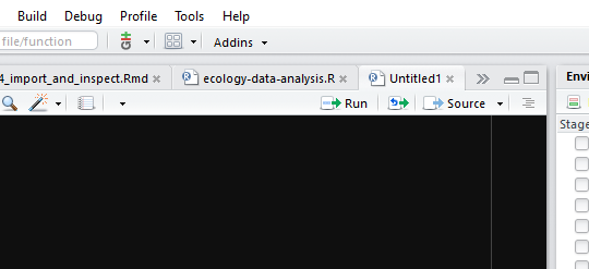
Figure 3.2: Scripts can be run by clicking the Source button.
You can run the entire script by clicking the Source button.
Or we can run chunks of code if we split our script into sections, see below.
3.4 Creating a R script
We first need to create a script that will form the basis of our analysis.
Go to the file menu and select New Files > R script. This should open the script editor pane.
Now let’s save the script, by going to File > Save and we should find ourselves prompted to save the script in our Project Directory.
Following the advice about naming things we can create a new R script
called 01-bspr-workshop-july-2018.
This name is machine readable (no spaces or special characters), human readable,
and works well with default ordering by beginning with 01.
3.5 Setting up our environment
At the head of our script it’s common to put a title, the name of the author
and the date, and any other useful information. This is created as comments
using the # at the start of each line.
It’s then usual to follow this by code to load the packages we need into our
our R environment using the library() function and providing the name of the
package we wish to load. Packages are collections of R functions.
Often we break the code up into regions by adding dashes (or equals symbols) to the comment line. This enables us to run chunks of the script separately from running the whole script when using our code.
Here is a typical head for a script:
# My workshop script
# 7th July 2018
# Alistair Bailey

# Load packages ----------------------------------------------------------------
library(plyr)
library(tidyverse)
library(gplots)
library(pheatmap)
library(gridExtra)
library(VennDiagram)
library(ggseqlogo)
3.5.1 Bioconductor
As an aside there are many proteomics specific R packages, these are generally found through Bioconductor which is a project that was initiated in 2001 to create tools for the analysis of high-throughput genomic data, but also includes other ’omics data tools (Gentleman et al. 2004, @huber2015).
Exploring Bioconductor is beyond our scope here, but well worth exploring for manipulation and analysis of raw data formats such as mzxml files.
3.6 Importing data
Assuming our data is in a flat format, we can import it into our
environment using the tidyverse readr package.
If our data was an excel file, we can use the tidyverse readxl package to
import the data, but it will remove any meta-data and each table in the excel
file will become a separate R object as per tidy data principles.
For the purposes of this workshop we have a csv (comma separated variable) file.
If you haven’t done so already
Click here to download the example data and save it to our project
directory. Check the Files pane to see it’s there.
We then import data and assign it to an object we’ll call data like so:
# Import example data ----------------------------------------------------------
# Import the example data with read_csv from the readr package
dat <- readr::read_csv("data/070718-proteomics-example-data.csv")
## Parsed with column specification:
## cols(
## protein_accession = col_character(),
## protein_description = col_character(),
## control_1 = col_double(),
## control_2 = col_double(),
## control_3 = col_double(),
## treatment_1 = col_double(),
## treatment_2 = col_double(),
## treatment_3 = col_double()
## )3.7 Exploring the data
3.7.1 glimpse, head and str
The first thing to do with any data set is to actually look at it. Here are
four ways to have look at the data in the Console: calling the object directly,
glimpse, head and str.
- We can just call the object and return it to the
Console, which may or may not be useful depending on the size and type of object we call.
2 .glimpse is a tidyverse function that tries to show us as much data in
a data.frame or tibble as possible, telling us the atomic types of
data in the table, the number of observations and the number of variables, and
importantly shows all the column variable names by transposing the table.
headis a base function that shows us the 6 lines of a R object by default.stris a base function that show the structure of a R object, so it provides a lot of information, but is not so easy to read.
The outputs for these four functions is shown below:
# call object
dat
## # A tibble: 7,702 x 8
## protein_accessi~ protein_descrip~ control_1 control_2 control_3
## <chr> <chr> <dbl> <dbl> <dbl>
## 1 VATA_HUMAN_P386~ V-type proton A~ 0.811 0.858 1.04
## 2 RL35A_HUMAN_P18~ 60S ribosomal p~ 0.367 0.385 0.409
## 3 MYH10_HUMAN_P35~ Myosin-10 OS=Ho~ 2.98 4.62 2.87
## 4 RHOG_HUMAN_P840~ Rho-related GTP~ 0.142 0.224 0.128
## 5 PSA1_HUMAN_P257~ Proteasome subu~ 1.07 0.945 0.803
## 6 PRDX5_HUMAN_P30~ Peroxiredoxin-5~ 0.566 0.540 0.488
## 7 ACLY_HUMAN_P533~ ATP-citrate syn~ 5.00 4.22 5.03
## 8 VDAC2_HUMAN_P45~ Voltage-depende~ 1.35 1.33 1.14
## 9 LRC47_HUMAN_Q8N~ Leucine-rich re~ 0.927 0.770 1.17
## 10 CH60_HUMAN_P108~ 60 kDa heat sho~ 9.45 8.41 10.4
## # ... with 7,692 more rows, and 3 more variables: treatment_1 <dbl>,
## # treatment_2 <dbl>, treatment_3 <dbl># tidyverse glimpse function
glimpse(dat)## Observations: 7,702
## Variables: 8
## $ protein_accession <chr> "VATA_HUMAN_P38606", "RL35A_HUMAN_P18077",...
## $ protein_description <chr> "V-type proton ATPase catalytic subunit A ...
## $ control_1 <dbl> 0.8114, 0.3672, 2.9815, 0.1424, 1.0748, 0....
## $ control_2 <dbl> 0.8575, 0.3853, 4.6176, 0.2238, 0.9451, 0....
## $ control_3 <dbl> 1.0381, 0.4091, 2.8709, 0.1281, 0.8032, 0....
## $ treatment_1 <dbl> 0.6448, 0.4109, 7.1670, 0.1643, 0.7884, 0....
## $ treatment_2 <dbl> 0.7190, 0.4634, 2.0052, 0.2466, 0.8798, 1....
## $ treatment_3 <dbl> 0.4805, 0.3561, 0.8995, 0.1268, 0.7631, 0....# head function
head(dat)## # A tibble: 6 x 8
## protein_accessi~ protein_descrip~ control_1 control_2 control_3
## <chr> <chr> <dbl> <dbl> <dbl>
## 1 VATA_HUMAN_P386~ V-type proton A~ 0.811 0.858 1.04
## 2 RL35A_HUMAN_P18~ 60S ribosomal p~ 0.367 0.385 0.409
## 3 MYH10_HUMAN_P35~ Myosin-10 OS=Ho~ 2.98 4.62 2.87
## 4 RHOG_HUMAN_P840~ Rho-related GTP~ 0.142 0.224 0.128
## 5 PSA1_HUMAN_P257~ Proteasome subu~ 1.07 0.945 0.803
## 6 PRDX5_HUMAN_P30~ Peroxiredoxin-5~ 0.566 0.540 0.488
## # ... with 3 more variables: treatment_1 <dbl>, treatment_2 <dbl>,
## # treatment_3 <dbl># str function
str(dat)## Classes 'spec_tbl_df', 'tbl_df', 'tbl' and 'data.frame': 7702 obs. of 8 variables:
## $ protein_accession : chr "VATA_HUMAN_P38606" "RL35A_HUMAN_P18077" "MYH10_HUMAN_P35580" "RHOG_HUMAN_P84095" ...
## $ protein_description: chr "V-type proton ATPase catalytic subunit A OS=Homo sapiens GN=ATP6V1A PE=1 SV=2" "60S ribosomal protein L35a OS=Homo sapiens GN=RPL35A PE=1 SV=2" "Myosin-10 OS=Homo sapiens GN=MYH10 PE=1 SV=3" "Rho-related GTP-binding protein RhoG OS=Homo sapiens GN=RHOG PE=1 SV=1" ...
## $ control_1 : num 0.811 0.367 2.982 0.142 1.075 ...
## $ control_2 : num 0.858 0.385 4.618 0.224 0.945 ...
## $ control_3 : num 1.038 0.409 2.871 0.128 0.803 ...
## $ treatment_1 : num 0.645 0.411 7.167 0.164 0.788 ...
## $ treatment_2 : num 0.719 0.463 2.005 0.247 0.88 ...
## $ treatment_3 : num 0.48 0.356 0.899 0.127 0.763 ...
## - attr(*, "spec")=
## .. cols(
## .. protein_accession = col_character(),
## .. protein_description = col_character(),
## .. control_1 = col_double(),
## .. control_2 = col_double(),
## .. control_3 = col_double(),
## .. treatment_1 = col_double(),
## .. treatment_2 = col_double(),
## .. treatment_3 = col_double()
## .. )To see the data in a spreadsheet fashion use View(dat), note the capital V
and a new tab will open. This can also be launched from the Environment tab by
clicking on dat.
Although this provides us with some useful information, such as the number of observations and variables, to understand more plotting the data will be helpful as we’ll see in Section 5.3.
3.7.2 Summary statisitics
Another useful way to quickly get a sense of the data is to use the summary
function, which will return summary of the spread of the data and importantly
if there are missing values. We can see immediately below that the experimental
replicates have different distributions, and missing values that we need to
deal with in Chapter 5.
summary(dat)## protein_accession protein_description control_1 control_2
## Length:7702 Length:7702 Min. : 0.001 Min. : 0.000
## Class :character Class :character 1st Qu.: 0.143 1st Qu.: 0.132
## Mode :character Mode :character Median : 0.345 Median : 0.322
## Mean : 0.933 Mean : 0.845
## 3rd Qu.: 0.959 3rd Qu.: 0.845
## Max. :31.944 Max. :31.697
## NA's :4888 NA's :4828
## control_3 treatment_1 treatment_2 treatment_3
## Min. : 0.001 Min. : 0.000 Min. : 0.002 Min. : 0.002
## 1st Qu.: 0.149 1st Qu.: 0.112 1st Qu.: 0.135 1st Qu.: 0.101
## Median : 0.388 Median : 0.286 Median : 0.319 Median : 0.254
## Mean : 0.977 Mean : 0.795 Mean : 0.856 Mean : 0.675
## 3rd Qu.: 0.999 3rd Qu.: 0.780 3rd Qu.: 0.880 3rd Qu.: 0.682
## Max. :31.320 Max. :41.686 Max. :28.234 Max. :21.428
## NA's :5087 NA's :4739 NA's :4902 NA's :5074References
Gentleman, Robert C, Vincent J Carey, Douglas M Bates, Ben Bolstad, Marcel Dettling, Sandrine Dudoit, Byron Ellis, et al. 2004. “Bioconductor: Open Software Development for Computational Biology and Bioinformatics.” Genome Biology 5 (10): R80. https://doi.org/10.1186/gb-2004-5-10-r80.